15.2.6 Algorithms (Fit Linear with X Error)Ref-Linear-XErr
The Fitting Model
For given dataset , (\sigma_{x_i},\sigma_{y_i}), i=1,2,\ldots n") , where X is the independent variable and Y is the dependent variable, and , where X is the independent variable and Y is the dependent variable, and ") are Errors for X, Y, respectively. -- Fit Linear with X Error fits the data to a model of the following form: are Errors for X, Y, respectively. -- Fit Linear with X Error fits the data to a model of the following form:
Fit Control
Computation Method
- York Method
- York Method is the computation method of D. York, described in Unified equations for the slope, intercept, and standard error of the best straight line
- FV Method
- FV Method is the computation method of Giovanni Fasano & Roberto Vio, described in Fittng a Straight Line with Errors on Both Coordinates.
- Deming Method
- Deming regression is the maximum likelihood estimation of an errors-in-variables model, the X/Y errors are assumed to be independent identically distributed.
- Correlation Between X and Y Errors
- Correlation Between X and Y Errors
 (For York method only) (For York method only)
- Standard Deviation of X/Y
- Standard Deviation of X/Y (For Deming method only)
Quantities (York Method)
When you perform a linear fit, you generate an analysis report sheet listing computed quantities. The Parameters table reports model slope and intercept (numbers in parentheses show how the quantities are derived):
Fit Parameters

Fitted Value and Standard Errors
Define  which involves the weight (error) for both x and y; which involves the weight (error) for both x and y;
Therein,  are weights of are weights of ") , is Correlation between X and Y Errors (i.e. , is Correlation between X and Y Errors (i.e.  and and  ), and ), and  . .
The slope of the fitted line for with no weighting (errors) is the initial value for  . They should be solved iteratively, until successive estimates of agree within desired tolerance. . They should be solved iteratively, until successive estimates of agree within desired tolerance.
The concise equations which estimate parameters  and and  for the best-fit line with X_Y errors are: for the best-fit line with X_Y errors are:
where  . .
U and V are the deviation for X and Y:

and
The corresponding variation  and standard error and standard error  for parameter is: for parameter is:
where  , ,  is the expectation value of is the expectation value of  , and , and  . .
The standard error for parameters is final given by:
where  is: is:
t-Value and Confidence Level
If the regression assumptions hold, we have:
The t-test can be used to examine whether the fitting parameters are significantly different from zero, which means that we can test whether  (if true, this means that the fitted line passes through the origin) or (if true, this means that the fitted line passes through the origin) or  . The hypotheses of the t-tests are: . The hypotheses of the t-tests are:
   
The t-values can be computed by:
With the computed t-value, we can decide whether or not to reject the corresponding null hypothesis. Usually, for a given confidence level  , we can reject , we can reject  when when  . Additionally, the p-value, or significance level, is reported with a t-test. We also reject the null hypothesis if the p-value is less than . . Additionally, the p-value, or significance level, is reported with a t-test. We also reject the null hypothesis if the p-value is less than .
Prob>|t|
The probability that in the t test above is true.
where tcdf(t, df) computes the lower tail probability for the Student's t distribution with df degree of freedom.
LCL and UCL
From the t-value, we can calculate the \times 100\%") Confidence Interval for each parameter by: Confidence Interval for each parameter by:
where  and and  is short for the Upper Confidence Interval and Lower Confidence Interval, respectively. is short for the Upper Confidence Interval and Lower Confidence Interval, respectively.
CI Half Width
The Confidence Interval Half Width is:
where UCL and LCL is the Upper Confidence Interval and Lower Confidence Interval, respectively.
For more information ,see Reference 1 (below).
Fit Statistics
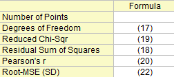
Degrees of Freedom
n is total number of points
Residual Sum of Squares
Reduced Chi-Sqr
Pearson's r
In simple linear regression, the correlation coefficient between x and y, denoted by r, equals to:
 can be computed as: can be computed as:
Root-MSE (SD)
Root mean square of the error, or residual standard deviation, which equals to:
Covariance and Correlation Matrix
The Covariance matrix of linear regression is calculated by:
The correlation between any two parameters is:
Quantities (FV Method)
FV Method is the computation method of Giovanni Fasano & Roberto Vio, described in Fittng a Straight Line with Errors on Both Coordinates.
The weighting is defined as:
The slope of the fitted line for with no weighting (errors) is .
Let
by minimizing the sum ^2}") , we can get the estimate value , we can get the estimate value  and by setting the partial derivatives to 0. and by setting the partial derivatives to 0.
where
should be solved iteratively, until successive estimates of agree within desired tolerance.
For each parameter standard error, please refer to Linear Regression Model
For more information ,see Reference 2 (below).
Quantities (Deming Method)
When you perform a linear fit, you generate an analysis report sheet listing computed quantities. The Parameters table reports model slope and intercept (numbers in parentheses show how the quantities are derived):
Fit Parameters

Deming regression is used for situation where both x and y are subjected to measurement error.
Assume are independent identically distributed with ") , and that are independent identically distributed with , and that are independent identically distributed with ") , where , where ") denotes the normal distribution with mean 0 and standard deviation denotes the normal distribution with mean 0 and standard deviation  . If . If  , it’s orthogonal regression.
The weighted sum of squared residuals of the model is minimized: , it’s orthogonal regression.
The weighted sum of squared residuals of the model is minimized:
Fitted Value and Standard Errors
We can solve the parameters:
where:
and:
The corresponding variation for parameters is:
The standard error for parameters can be estimated by:
and
t-Value and Confidence Level
If the regression assumptions hold, we have:
The t-test can be used to examine whether the fitting parameters are significantly different from zero, which means that we can test whether (if true, this means that the fitted line passes through the origin) or . The hypotheses of the t-tests are:
-
-
The t-values can be computed by:
With the computed t-value, we can decide whether or not to reject the corresponding null hypothesis. Usually, for a given confidence level , we can reject when . Additionally, the p-value, or significance level, is reported with a t-test. We also reject the null hypothesis if the p-value is less than .
Prob>|t|
The probability that in the t test above is true.
where tcdf(t, df) computes the lower tail probability for the Student's t distribution with df degree of freedom.
LCL and UCL
From the t-value, we can calculate the Confidence Interval for each parameter by:
where and is short for the Upper Confidence Interval and Lower Confidence Interval, respectively.
CI Half Width
The Confidence Interval Half Width is:
where UCL and LCL is the Upper Confidence Interval and Lower Confidence Interval, respectively.
For more information ,see Reference 1 (below).
Fit Statistics
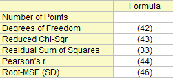
Degrees of Freedom
n is total number of points
Residual Sum of Squares
See formula (33)
Reduced Chi-Sqr
Pearson's r
In simple linear regression, the correlation coefficient between x and y, denoted by r, equals to:
can be computed as:
Root-MSE (SD)
Root mean square of the error, which equals to:
Covariance and Correlation Matrix
The Covariance matrix of linear regression is calculated by:
The correlation between any two parameters is:
Residual Plots
Residual vs. Independent
Scatter plot of residual  vs. indenpendent variable vs. indenpendent variable  , each plot is located in a seperate graphs. , each plot is located in a seperate graphs.
Residual vs. Predicted Value
Scatter plot of residual vs. fitted results 
Residual vs. Order of the Data
 vs. sequence number vs. sequence number 
Histogram of the Residual
The Histogram plot of the Residual
Residual Lag Plot
Residuals vs. lagged residual }") . .
Normal Probability Plot of Residuals
A normal probability plot of the residuals can be used to check whether the variance is normally distributed as well. If the resulting plot is approximately linear, we proceed to assume that the error terms are normally distributed. The plot is based on the percentiles versus ordered residual, and the percentiles is estimated by
}{(n+\frac{1}{4})}")
where n is the total number of dataset and i is the i th data.
Also refer to Probability Plot and Q-Q Plot
Reference
- York D, Unified equations for the slope, intercept, and standard error of the best straight line, American Journal of Physics, Volume 72, Issue 3, pp. 367-375 (2004).
- G. Fasano and R. Vio, "Fitting straight lines with errors on both coordinates", Newsletter of Working Group for Modern Astronomical Methodology, No. 7, 2-7, Sept. 1988.
|