15.2.5 Algorithms (Linear Regression)LR-Algorithm
The Linear Regression Model
Simple Linear Regression Model
For a given dataset ,i=1,2,\ldots n") -- where x is the independent variable and y is the dependent variable, -- where x is the independent variable and y is the dependent variable,  and and  are parameters, and are parameters, and  is a random error term with mean is a random error term with mean  and variance and variance  -- linear regression fits the data to a model of the following form: -- linear regression fits the data to a model of the following form:
The least squares estimation is used to minimize the sum of the n squared deviations
the estimated parameters of linear model can be computed as:
where:
and
| Note: When the intercept is excluded from the model, the coefficients are calculated using the uncorrected formula.
|
Therefore, we estimate the regression function as follows:
the residual  is defined as: is defined as:
formula in (2) is to be minimized equaling to residual sum of squares
when the least squares estimators  and and  are used for estimating and . are used for estimating and .
Fit Control
Errors as Weight
In above section, we assume that there is constant variance in the errors. However, when we fit the experimental data, we may need to take the instrument error (which reflect the accuracy and precision of a measuring instrument) into account in fitting process. Therefore, the assumption of constant variance in the errors is violated. Thus, we need to assume to be normally distributed with nonconstant variance, and the errors act as  , which can be used as weight in fitting. The weight is defined as: , which can be used as weight in fitting. The weight is defined as:
The fitting model is changed into:
The weight factors  can be given by three formulas: can be given by three formulas:
No Weighting
The error bar will not be treated as weight in calculation.
Direct Weighting
Instrumental
As for Instrumental weight, the value is inversely proportional to the instrumental errors, so a trial with small errors will have a larger weight because it is rather precise than some other trials with larger errors.
| Note: The errors as weight should be desiganited as "YError" column in worksheet.
|
|
Fix Intercept (at)
Fix intercept will set the y-intercept to a fixed value, meanwhile, the total degree of freedom will be n*=n-1 due to the intercept fixed.
Scale Error with sqrt(Reduced Chi-Sqr)
Scale Error with sqrt(Reduced Chi-Sqr) is available when fitting with weight. This option only affects the error on the parameters reported from the fitting process, and does not affect the fitting process or the data in any way.
By default, it is checked, and is taken into account when calculate error on the parameters, otherwise, will not be taken into account for error calculation.
Take Covariance Matrix as an example:
Scale Error with sqrt(Reduced Chi-Sqr):
Do not Scale Error with sqrt(Reduced Chi-Sqr):
For weighted fitting, ^{-1}\,\!") is used instead of is used instead of ^{-1}\,\!") . .
Fit Results
When you perform a linear fit, you generate an analysis report sheet listing computed quantities. The Parameters table reports model slope and intercept (numbers in parentheses show how the quantities are derived):
Fit Parameters

Fitted value
See formula (3)&(4)
The Parameter Standard Errors
For each parameter, the standard error can be obtained by:
where the sample variance  (or error mean square, (or error mean square,  ) can be estimated as follows: ) can be estimated as follows:
And RSS means the residual sum of square (or error sum of square, SSE), which is actually the sum of the squares of the vertical deviations from each data point to the fitted line. It can be computed as:
Note : Regarding  , if intercept is included in the model, , if intercept is included in the model,  . Otherwise, . Otherwise,  . .
|
t-Value and Confidence Level
If the regression assumptions hold, we have:
The t-test can be used to examine whether the fitting parameters are significantly different from zero, which means that we can test whether  (if true, this means that the fitted line passes through the origin) or (if true, this means that the fitted line passes through the origin) or  . The hypotheses of the t-tests are: . The hypotheses of the t-tests are:
   
The t-values can be computed by:
With the computed t-value, we can decide whether or not to reject the corresponding null hypothesis. Usually, for a given confidence level  , we can reject , we can reject  when when  . Additionally, the p-value, or significance level, is reported with a t-test. We also reject the null hypothesis if the p-value is less than . . Additionally, the p-value, or significance level, is reported with a t-test. We also reject the null hypothesis if the p-value is less than .
Prob>|t|
The probability that in the t test above is true.
where tcdf(t, df) computes the lower tail probability for the Student's t distribution with df degree of freedom.
LCL and UCL
From the t-value, we can calculate the \times 100\%") Confidence Interval for each parameter by: Confidence Interval for each parameter by:
where  and and  is short for the Upper Confidence Interval and Lower Confidence Interval, respectively. is short for the Upper Confidence Interval and Lower Confidence Interval, respectively.
CI Half Width
The Confidence Interval Half Width is:
where UCL and LCL is the Upper Confidence Interval and Lower Confidence Interval, respectively.
Fit Statistics
Key linear fit statistics are summarized in the Statistics table (numbers in parentheses show how quantities are computed):
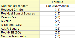
Degrees of Freedom
The Error degrees of freedom. Please refer to the ANOVA table for more details.
Residual Sum of Squares
The residual sum of squares, see formula (19).
Reduced Chi-Sqr
See formula (14)
R-Square (COD)
The quality of linear regression can be measured by the coefficient of determination (COD), or  , which can be computed as: , which can be computed as:
where TSS is the total sum of square, and RSS is the residual sum of square. The is a value between 0 and 1. Generally speaking, if it is close to 1, the relationship between X and Y will be regarded as very strong and we can have a high degree of confidence in our regression model.
Adj. R-Square
We can further calculate the adjusted as
R Value
The R value is the square root of :
Pearson's r
In simple linear regression, the correlation coefficient between x and y, denoted by r, equals to:
Root-MSE (SD)
Root mean square of the error, or residual standard deviation, which equals to:
Norm of Residuals
Equals to square root of RSS:
ANOVA Table
The ANOVA table of linear fitting is:
|
|
DF
|
Sum of Squares
|
Mean Square
|
F Value
|
Prob > F
|
| Model
|
1
|

|

|

|
p-value
|
| Error
|
n* - 1
|
RSS
|
MSE = RSS / (n* - 1)
|
|
|
| Total
|
n*
|
TSS
|
|
|
|
Note: If intercept is included in the model, n*=n-1. Otherwise, n*=n and the total sum of squares is uncorrected. If the slope is fixed,  = 0. = 0.
|
Where the total sum of square, TSS, is:
The F value here is a test of whether the fitting model differs significantly from the model y=constant.
The p-value, or significance level, is reported with an F-test. If the p-value is less than , the fitting model differs significantly from the model y=constant.
If fixing the intercept at a certain value, the p value for F-test is not meaningful, and it is different from that in linear regression without the intercept constraint.
Lack of fit table
To run the lack of fit test, you need to have repeated observations, namely, "replicate data" , so that at least one of the X values is repeated within the dataset, or within multiple datasets when concatenate fit mode is selected.
Notations used for fit with replicates data:
The sum of square in table below is expressed by:
The Lack of fit table of linear fitting is:
|
|
DF
|
Sum of Squares
|
Mean Square
|
F Value
|
Prob > F
|
| Lack of Fit
|
c-2
|
LFSS
|
MSLF = LFSS / (c - 2)
|
MSLF / MSPE
|
p-value
|
| Pure Error
|
n - c
|
PESS
|
MSPE = PESS / (n - c)
|
|
|
| Error
|
n*-1
|
RSS
|
|
|
|
Note:
If intercept is included in the model, n*=n-1. Otherwise, n*=n and the total sum of squares is uncorrected. If the slope is fixed, = 0.
c denotes the number of distinct x values. If intercept is fixed, DF for Lack of Fit is c-1.
|
Covariance and Correlation Matrix
The Covariance matrix of linear regression is calculated by:
The correlation between any two parameters is:
Outliers
The Outliers are those points whose absolute values in Studentized Residual plot are larger than 2.
>2")
Studentized Residual is introduced in Detecting outliers by transforming residuals.
Residual Analysis
 stands for the Regular Residual . stands for the Regular Residual .
Standardized
Studentized
Also known as internally studentized residual.
Studentized deleted
Also known as externally studentized residual.
In the equations for the Studentized and Studentized deleted residuals,  is the ith diagonal element of the matrix is the ith diagonal element of the matrix  : :
 means the variance is calculated based on all points but exclude the ith. means the variance is calculated based on all points but exclude the ith.
Confidence and Prediction Bands
For a particular value  , the , the \%") confidence interval for the mean value of confidence interval for the mean value of  at at  is: is:
And the prediction interval for the mean value of at is:
Confidence Ellipses
Assuming the pair of variables (X, Y) conforms to a bivariate normal distribution, we can examine the correlation between the two variables using a confidence ellipse. The confidence ellipse is centered at ( , , ), and the major semiaxis a and minor semiaxis b can be expressed as follow: ), and the major semiaxis a and minor semiaxis b can be expressed as follow:
For a given confidence level of \,\!") : :
- The confidence ellipse for the population mean is defined as:
- The confidence ellipse for prediction is defined as:
- The inclination angle of the ellipse is defined as:
Residual Plots
Resudial Type
Select one residual type among Regular, Standardized, Studentized, Studentized Deleted for Plots.
Residual vs. Independent
Scatter plot of residual  vs. indenpendent variable vs. indenpendent variable  , each plot is located in a seperate graphs. , each plot is located in a seperate graphs.
Residual vs. Predicted Value
Scatter plot of residual vs. fitted results  . .
Residual vs. Order of the Data
vs. sequence number 
Histogram of the Residual
The Histogram plot of the Residual
Residual Lag Plot
Residuals vs. lagged residual }") . .
Normal Probability Plot of Residuals
A normal probability plot of the residuals can be used to check whether the variance is normally distributed as well. If the resulting plot is approximately linear, we proceed to assume that the error terms are normally distributed. The plot is based on the percentiles versus ordered residual, and the percentiles is estimated by
}{(n+\frac{1}{4})}")
where n is the total number of dataset and i is the i th data. Also refer to Probability Plot and Q-Q Plot
|