17.1.1.1 The Statistics on Columns Dialog BoxDescStats-Dialog
Supporting Information
Recalculate
See Recalculating Analysis Results for details of the recalculation options.
Input
Exclude Empty Dataset
Check this check box to exclude empty dataset in calculation.
Exclude Text Dataset
Check this check box to exclude Text dataset in calculation.
Input Data
Specify the input data mode, indexed or raw.
Quantities
Moments
Let  be the be the  th sample and th sample and  be the th weight: be the th weight:
| N Total
|
Total number of data points, denoted by n
|
| N Missing
|
Number of missing values
|
| Mean
|
The mean (average) score
 . If there is no WEIGHT variable, the formula reduces to . If there is no WEIGHT variable, the formula reduces to  . .
|
| Standard deviation
|
^2/d}")
where 
Note: In OriginPro,  has 4 more options, which are defined in the Variance Divisor of Moment branch. has 4 more options, which are defined in the Variance Divisor of Moment branch.
|
| SE of Mean
|
Standard error of mean:

|
| Lower 95% CI of Mean
|
Lower limit of the 95% confidence interval of mean
}\frac s{\sqrt{n}}")
where }") is the is the ") critical value of the Student's t-statistic with n-1 degrees of freedom critical value of the Student's t-statistic with n-1 degrees of freedom
|
| Upper 95% CI of Mean
|
Upper limit of the 95% confidence interval of mean
}\frac s{\sqrt{n}}")
where is the critical value of the Student's t-statistic with n-1 degrees of freedom
|
| Variance
|

|
| Sum
|
 . If there is no WEIGHT variable, the formula reduces to . If there is no WEIGHT variable, the formula reduces to  . .
|
| Skewness
|
Skewness measures the degree of asymmetry of a distribution. It is defined as
(n-2)}\sum_{i=1}^n w_i^{\frac 32}(\frac{x_i-\bar{x}}s)^3 ,\mbox{for DF}")
^3,\mbox{for N}")
^3,\mbox{for WVR}")
Note: When the WDF or WS methods are chosen, skewness is returned as a missing value.
|
| Kurtosis
|
Kurtosis depicts the degree of peakedness of a distribution.
}{(n-1)(n-2)(n-3)}\sum_{i=1}^n w_i^2(\frac{x_i-\bar{x}}s)^4-\frac{3(n-1)^2}{(n-2)(n-3)},\mbox{for DF}")
^4 -3,\mbox{for N}")
^4 -3,\mbox{for WVR}")
Note: When the WDF or WS methods are chosen, kurtosis is returned as a missing value.
|
| Uncorrected Sum of Squares
|

|
| Corrected Sum of Squares
|
^2")
|
| Coefficient of Variance
|

|
| Mean absolute Deviation
|

|
| SD times 2
|
Standard deviation times 2.

|
| SD times 3
|
Standard deviation times 3.

|
| Geometric Mean
|
 ^{\frac 1n}")
Note:: Weights are ignored for the geometric mean.
|
| Geometric SD
|
The geometric standard deviation
}") Where std is the unweighted sample standard deviation.
Where std is the unweighted sample standard deviation.
Note: Weights are ignored for the geometric standard deviation.
|
| Mode
|
The mode is the element that appears most often in the data range. If multiple modes are found, the smallest will be chosen.
|
| Sum of Weights
|

|
| Harmonic Mean
|
harmonic mean (sometimes called the subcontrary mean)
without weight: ^{-1}}n\right)^{-1}")
with weight: ^{-1}")
if any  or weight is negative, return missing; if any or weight is 0, return 0. or weight is negative, return missing; if any or weight is 0, return 0.
|
Quantiles
Quantiles are values from the data, below which is a given proportion of the data points in a given set. For example, 25% of data points in any set of data lay below the first quartile, and 50% of data points in a set lay below the second quartile, or median.
Sort the input dataset in ascending order. Let \,") be the th element of the reordered dataset be the th element of the reordered dataset
| Minimum
|
}\,")
|
| Index of Minimum
|
The index number of Minimum in the original (input) dataset
|
| 1st Quartile (Q1)
|
First (25%) quantile, Q1. See Interpolation of quantiles for computational methods
|
| Median
|
Median or second (50%) quantile, Q2. See Interpolation of quantiles for computational methods
|
| 3rd Quartile (Q3)
|
Third (75%) quantile, Q3. Interpolation of quantiles for computational methods
|
| Maximum
|
}\,")
|
| Index of Maximum
|
The index number of Maximum in the original (input) dataset
|
| Interquartile Range (Q3-Q1)
|

|
| Range (Maximum-Minimum)
|
Maximum - Minimum
|
| Custom Percentile(s)
|
Request computation of custom percentiles.
|
| Percentile list
|
This option is only available when Custom Percentile(s) is checked. Percentiles are computed for all the values listed.
|
| Median Absolute Deviation
|
For a univariate data set X1, X2, ..., Xn, the MAD is defined as the median of the absolute deviations from the data's median:
|)\,")
that is, starting with the residuals (deviations) from the data's median, the MAD is the median of their absolute values.
|
| Robust Coefficient of Variation
|
)/Median\,")
|
Extreme Values
Return extreme values. Extreme values are the lst highest and the lst lowest values.

where n is the length of the dataset.
Computation Control
Weight Method
Choose weighting methods for input data.
Variance Divisor of Moment
Controls computation of variance divisor d.
| DF
|
Degrees of freedom

|
| N
|
Number of non-missing observations

|
| WDF
|
Sum of weights DF

|
| WS
|
Sum of weights

|
| WVR
|

|
Interpolation of quantiles
Methods for calculating Q1, Q2, and Q3:
Let the th percentile be y, set , and let , and let
p=j+g, & \mbox{for Weighted Average Right } \\
np=(j+g),& \mbox{for other methods }
\end{cases}")
where j is the integer part of np, and g is the fractional part of np, then different methods define the  percentile, y, as described by the following: percentile, y, as described by the following:
|
Note: if weights are specified, Weighted Percentiles are calculated. The pth weighted percentile y is computed from the Empirical Distribution Function with Averaging:
}+x_{(i+1)}),& \mbox{if } \sum_{j=1}^i w_j=pw \\
x_{(i+1)},& \mbox{if } \sum_{j=1}^{i} w_j<pw<\sum_{j=1}^{i+1}w_j\\
x_{(1)},& \mbox{if } \ pw<w_1 \\
x_{(n)},& \mbox{if } \ pw<w_n \\
\end{cases}")
|
Output
 | Beginning with Origin 2022, input column Format of a Group column will be preserved in the output sheet (e.g. DescStatsQuantities). For instance, when outputting stats on a column of Date-Time data, column Format will be set as Date-Time in the output sheet (previously, the column would have been formatted as Text). You can restore the old behavior by setting @SCCSF = 0. For information on changing the value of a system variable, see FAQ-708 How do I permanently change the value of a system variable?
|
| Graph
|
Control arrangement of resulting plots.
- Arrange Graphs into Columns
- Specify number of columns to arrange output graphs.
- Arrange Plots of Same Type in One Graph
- Check to plot all graphs of same type in one graph window.
|
| Dataset Identifier
|
Choose an identifier for the source datasets.
- Identifier
- Select from the list:
-
- Use the range syntax.
- Use the workbook long name.
- Use the worksheet name.
- Use column Long Name if it exists, otherwise Short Name.
- Use column Short Name.
- Use column Long Name.
- Use column Units.
- Use column Comments.
- Use custom formats to define a data identifier. For usage information, please refer to Advanced legend text customizations.
- Show Identifier in Flat Sheet
- Use the dataset identifier in resulting flat sheet(s).
|
| Report Tables
|
Destination for report worksheet tables.
- Book
- The target workbook.
- <none>: Do not output report worksheet tables.
- <source>: The source data workbook.
- <new>: A new workbook.
- <existing>: An existing workbook.
- BookName
- The target workbook. Must be source (uneditable), new or existing (editable), otherwise blank.
- Sheet
- The target worksheet, always <new>.
- SheetName
- Name of the target sheet.
- Results Log
- Output the report to the Results Log.
- Script Window
- Output the report to the Script Window.
- Notes Window
- Specify the target Notes window:
- <none>: Do not output to a Notes window.
- <new>: Output to a new Notes window.
|
| Quantities
|
Specifies the destination of quantities
- Book
- Specifies the destination workbook
- <none>: Do not output quantities
- <source>: The source data workbook
- <report>: The Report Tables workbook
- <new>: A new workbook.
- <existing>: A specified existing workbook
- BookName
- The target workbook. Must be source (uneditable), new or existing (editable), otherwise blank.
- Sheet
- <new>: A new worksheet.
- <source>: The source data worksheet
- <existing>: A specified existing worksheet
- SheetName
- Name of the target sheet.
|
| Optional Report Tables
|
Specifies what is output to report worksheet
- Notes
- Notes table
- Input Data
- Table for input data
- Masked Data
- Table for masked data
- Missing Data
- Table for missing data
|
Plots
| Histograms
|
Outputs a histogram to the result sheet.
When this box is selected, the branch is expanded. In this branch,
- The Data Height drop-down determines the Y axis of the histogram.
- Count: Y axis displays bin counts.
- Relative Frequency: Y axis displays individual bin counts divided by total count.
- Density: Y axis displays relative frequency (no. of observations in a given bin) divided by bin width.
- The Automatic Binning check box is selected by default. Bin Size, Number of Bins, Begin, End are shown automatically when Automatic Binning is clear.
| Note: If the input data are in multiple columns, Automatic Binning will use independent settings for each column and thus the binning and axis range may vary a lot. In this case, Origin will display non-editable limit values for each column. If the Automatic Binning check box is cleared, these items will be editable with an initial value.
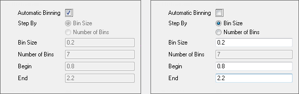
After you edit the value of Bin Size, Beginning and/or End, the Number of Bins will be computed automatically.
Number of Bins and Bin Size can be switched by Step By.
Number of Bins = (Begin - End) / Bin Size
|
|
| Box Charts
|
Outputs a box chart to the report sheet. If the input data has a group column, the box chart is grouped accordingly. If the group column is Set as Categorical, the box chart will be plotted according to categorical order customized through (Column Properties) Categories tab from grouping range.
|
|