15.4.1 Additional Information of R-squareDetails_of_R_square
How good is the fit? One obvious metric is how close the fitted curve is to the actual data points. From the previous section, we know that the residual sum of square (RSS) or the reduced chi-square value is a quantitative value that can be used to evaluate this kind of distance. However, the value of residual sum of square (RSS) varies from dataset to dataset, making it necessary to rescale this value to a uniform range. On the other hand, one may want to use the mean of y value to describe the data feature. If this is the case, the fitted curve is a horizontal line , and the predictor x, cannot linearly predict the y value. To verify this, we first calculate the variation between data points and the mean, the "total sum of squares" about the mean, by , and the predictor x, cannot linearly predict the y value. To verify this, we first calculate the variation between data points and the mean, the "total sum of squares" about the mean, by
^2 \,\!")
In least-squares fitting, the TSS can be divided into two parts: the variation explained by regression and that not explained by regression:
- The regression sum of squares, SSreg, is the portion of the variation that is explained by the regression model.
|
^2 \,\!")
|
- The residual sum of squares, RSS, is the portion that is not explained by the regression model.
|
^2 \,\!")
|
Clearly, the closer the data points are to the fitted curve, the smaller the RSS and the greater the proportion of the total variation that is represented by the SSreg. Thus, the ratio of SSreg to TSS can be used as one measure of the quality of the regression model. This quantity -- termed the coefficient of determination -- is computed as:

From the above equation, we can see that when using a good fitting model,  should vary between 0 and 1. A value close to 1 indicates that the fit is a good one. should vary between 0 and 1. A value close to 1 indicates that the fit is a good one.
Mathematically speaking, the degrees of freedom will affect . That is, when adding variables in the model, will rise, but this does not imply a better fit. To avoid this effect, we can look at the adjusted :

From the equation, we can see that adjusted overcomes the rise in , especially when fitting a small sample size (n) by multiple predictor (k) model. Though we usually term the coefficient of determination as "R-square", it is actually not a "square" value of R. For most cases, it is a value between 0 and 1, but you may also find negative R^2 when the fit is poor. This occurs because the equation to calculate is  . The second term will be greater then 1, when a bad model is used. . The second term will be greater then 1, when a bad model is used.
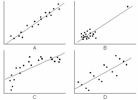
However, using or adjusted is not sufficient. For example, in the following graph, the fitted curve shown in plot B-D might have a high value, but apparently the models are wrong. So it is necessary to diagnose the regression result by the Residual Analysis.
R-Square in Linear Fit
Linear Fit for Intercept Included
When intercept is included in linear fit , it follows the relation:
^2 = \sum_{i=1}^n (y_i-f(x_i))^2 + \sum_{i=1}^n (f(x_i)-\bar{y})^2")
where  \; i=1..n \;") are fitting data, are fitting data,  denotes the mean of the dependent variable and denotes the mean of the dependent variable and  \;") is the fitted value. is the fitted value.
The left hand side in the above equation is the total sum of squares, i.e.
^2")
The first term on the right is the residual sum of squares, i.e.
)^2")
And the second term on the right is the sum of squares due to regression, i.e.
-\bar{y})^2")
Hence TSS = RSS + SSR.
And the coefficient of determination (R-Square) is defined by the ratio of SSR to TSS:
)^2}{\sum_{i=1}^n (y_i-\bar{y})^2}")
Therefore R-Square measures the proportion of variation of the dependent variable about the mean explained by the fitting when intercept is included.
Linear Fit for Fixed Intercept
However, when intercept is fixed in linear fit, the above relation in Linear Fit for Intercept Included is not satisfied. For a poor fit, it may result in a negative R-Square value using the definition in Linear Fit for Intercept Included. And this is not reasonable.
When intercept is fixed in linear fit, it follows the relation below:
)^2 + \sum_{i=1}^n (f(x_i))^2")
Then TSS and SSR need be redefined, and RSS is unchanged.

)^2")
And the coefficient of determination (R-Square) is redefined as follows:
)^2}{\sum_{i=1}^n y_i^2}")
In this way, the R-Square value will always be non-negative. And R-Square measures the proportion of variation of the dependent variable around the value zero explained by the fitting when intercept is fixed.
|