15.4.4 Residual Plot AnalysisResidual-Plot-Analysis
The residual is defined as:

The regression tools below provide the options to calculate the residuals and output the customized residual plots:
To perform residual analysis in the fitting tools
All the fitting tools has two tabs, In the Residual Analysis tab, you can select methods to calculate and output residuals, while with the Residual Plots tab, you can customize the residual plots
Residual plots can be used to assess the quality of a regression. Currently, six types of residual plots are supported by the linear fitting dialog box:
- Residual vs. Independent
- Residual vs. Predicted Value
- Residual vs. Order of the Data
- Histogram of the Residual
- Residual Lag Plot
- Normal Probability Plot of Residuals
These residual plots can be used to assess the quality of the regression. You can examine the underlying statistical assumptions about residuals such as constant variance, independence of variables and normality of the distribution. For these assumptions to hold true for a particular regression model, the residuals would have to be randomly distributed around zero.
Different types of residual plots can be used to check the validity of these assumptions and provide information on how to improve the model. For example, the scatter plot of the residuals will be disordered if the regression is good. The residuals should not show any trend. A trend would indicate that the residuals were not independent. On the other hand, a histogram plot of the residuals should exhibit a symmetric bell-shaped distribution, indicating that the normality assumption is likely to be true.
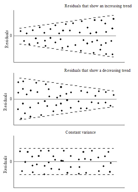
Checking the error variance
A residuals plot (see the picture below) which has an increasing trend suggests that the error variance increases with the independent variable; while a distribution that reveals a decreasing trend indicates that the error variance decreases with the independent variable. Neither of these distributions are constant variance patterns. Therefore they indicate that the assumption of constant variance is not likely to be true and the regression is not a good one. On the other hand, a horizontal-band pattern suggests that the variance of the residuals is constant.
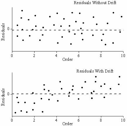
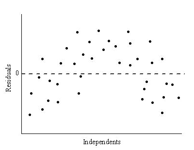
Checking the process drift
The Residual vs. Order of the Data plot can be used to check the drift of the variance (see the picture below) during the experimental process, when data are time-ordered. If the residuals are randomly distributed around zero, it means that there is no drift in the process.
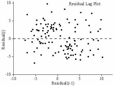
Checking independence of the error term
The Residual Lag Plot (see the picture below), constructed by plotting residual (i) against residual (i-1), is useful for examining the dependency of the error terms. Any non-random pattern in a lag plot suggests that the variance is not random.
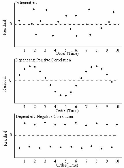
If the data being analyzed is time series data (data recorded sequentially), the Residual vs. Order of the Data plot will reflect the correlation between the error term and time. Fluctuating patterns around zero will indicate that the error term is dependent.
Residual Lag Plot showing that the error term is independent.
Residual plots for time series data.
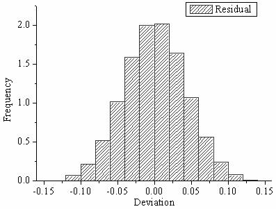
Checking normality of variance
The Histogram of the Residual can be used to check whether the variance is normally distributed. A symmetric bell-shaped histogram which is evenly distributed around zero indicates that the normality assumption is likely to be true. If the histogram indicates that random error is not normally distributed, it suggests that the model's underlying assumptions may have been violated.
Histogram of the Residuals showing that the deviation is normally distributed.
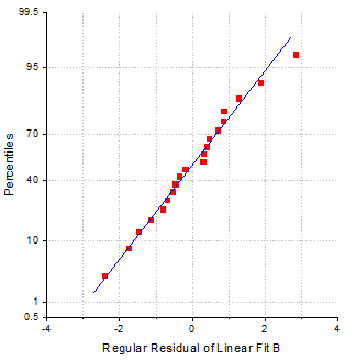
A normal probability plot of the residuals can be used to check whether the variance is normally distributed as well. If the resulting plot is approximately linear, we proceed assuming that the error terms are normally distributed. The plot is based on the percentiles versus ordered residual, the percentiles is estimated by
}{(n+\frac{1}{4})}")
where n is the total number of dataset and i is the i th data. The normal probability plot of the residuals is like this:
Normal Probability Plot of the Residuals
Improving the regression model using residuals plots
The pattern structures of residual plots not only help to check the validity of a regression model, but they can also provide hints on how to improve it. For example, a curved pattern in the Residual vs. Independent plot suggests that a higher order term should be introduced to the fitting model.
This is only one example and, certainly, there is much more that can be surmised from studying residual plot patterns. We suggest that you refer to the statistical references given at the end of this chapter/section, for more information.
Detecting outliers by transforming residuals
When looking for outliers in your data, it may be useful to transform the residuals to obtain standardized, studentized or studentized deleted residuals. These transformed residuals are computed as follows:
Standardized

Studentized
Also known as internally studentized residual.

Studentized deleted
Also known as externally studentized residual.

In the equations for the Studentized and Studentized deleted residuals,  is the ith diagonal element of the matrix, P: is the ith diagonal element of the matrix, P:
^{-1}F^{\prime }")
where F is the partial derivatives matrix for a nonlinear regression model.
In a linear regression model, the independent matrix, X, is simply equal to F:
^{-1}X^{\prime }")
As an example of the use of transformed residuals, standardized residuals rescale residual values by the regression standard error, so if the regression assumptions hold -- that is, the data are distributed normally -- about 95% data points should fall within 2σ around the fitted curve. Consequently, 95% of the standardized residuals will fall between -2 and +2 in the residual plot.
These variations of residual plots are very useful in detecting outliers. For example, in the Standardized Residual vs. Independent Plots, the residuals are rescaled by the regression standard error. If the regression assumption holds, that is, the data is distributed normally, about 95% data points should be located within 2σ around the fitted curve, and consequently, 95% of the standardized residuals will fall between -2 and +2, as shown in the graph below.
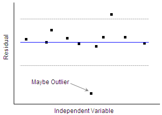
So residuals out of this range should be more closely examined, because these points may be outliers.
Residual contour plots for surface fitting
When fitting a surface with an OriginPro built-in function, a contour plot of residuals in the XY plane is produced. Contour intervals are determined by the sigma value (the model error). As in the case of 2D fitting, a good fit of the regression surface should produce no recognizable patterns in the contour plot of the residuals
|