2.8.14 interp2
Menu Information
Interpolate Z from XY
Brief Information
Perform interpolation on XYZ data at a given set of XY values
Additional Information
Minimum Origin Version Required: 9.1 SR0
Command Line Usage
1.interp2 ixy:=[XYZRandomGaus]"XYZ Random Gaussian"!(D,E) ir:=[XYZRandomGaus]"XYZ Random Gaussian"!(A,B,C) method:=rk pts:=3 smooth:=4;
X-Function Execution Options
Please refer to the page for additional option switches when accessing the x-function from script
Variables
Display
Name
|
Variable
Name
|
I/O
and
Type
|
Default
Value
|
Description
|
| XY Values to Interpolate
|
ixy
|
Input
XYRange
|
<unassigned>
|
Specify the input XY range for the given XY values.
|
| Input
|
ir
|
Input
XYZRange
|
<active>
|
Specify the input XYZ range for the group of XYZ data.
|
| Method
|
method
|
Input
int
|
0
|
Specify the interpolation method to be used. 8 methods are available.
Option list:
- nr:Nearest
- rk:Random Kriging
- rc:Renka Renka Cline
- rs:Random Shepard
- tps:Random TPS
- sp:Spline
- ta:Triangle
- wa:Weight Average
More details can be found in the Algorithm section below.
|
| Search Radius
|
radius
|
Input
double
|
2
|
Specify a search radius. Only available when the method is either Random Kriging or Weight Average.
|
| Minimum Points
|
pts
|
Input
int
|
2
|
Specify a minimum number of points. Only available when the method is Random Kriging.
|
| Smoothing Factor
|
smooth
|
Input
double
|
<unassigned>
|
Specify a Kriging or Spline smoothing factor. Only available when the method is either Random Kriging or Spline.
|
| Input Weight
|
weight
|
Input
vector
|
|
Specify a vector as the weight. Only available when the method is Spline.
|
| Weight Function Locality Factor
|
nw
|
Input
int
|
9
|
Specify a weight function locality factor. Only available when the method is Random Shepard.
|
| Quadratic Interpolant Locality Factor
|
nq
|
Input
int
|
18
|
Specify a quadratic interpolant locality factor. Only available when the method is Random Shepard.
|
| Result of Interpolation
|
oz
|
Output
vector
|
<new>
|
Specify where to output the interpolation result.
|
Description
This X-Function is used to interpolate a group of existing xyz data to find z value for given (x,y), using one of eight (8) methods: Nearest, Random Kriging, Random Renka Cline, Random Shepard, Random TPS, Spline, Triangle and Weight Average.
In order to interpolate z from xy, using the interp2 X-Function:
- In Script Window, run
interp2 -d;
to open the interp2 dialog box.
- Pick data (x,y) from worksheet as XY Values To Interpolate, and a range of xyz data as Input for interpolation.
- Select a Method from the drop-down menu.
- Assign destination columns as Result of Interpolation.
Algorithm
Interp2 provides estimation of a variable at an unmeasured location from observed values at surrounding locations. There are 8 methods used in X-Function Interp2, the correspondence for each method and algorithm are listed in table below.
| Methods
|
Algorithm
|
| Nearest
|
Nearest-neighbor interpolation
|
| Random Kriging
|
Ordinary Kriging interpolation
|
| Random Renka Cline
|
Triangle-based Renka Cline interpolation
|
| Random Shepard
|
Modification of Shepard’s method interpolation
|
| Random TPS
|
Random TPS interpolation
|
| Spline
|
Bicubic B-spline interpolation
|
| Triangle
|
Triangle-based Renka Cline interpolation
|
| Weight Average
|
Inverse Distance Weighting interpolation
|
Nearest neighbor interpolation
In the nearest neighbor algorithm, it finds the nearest point of the given to-be-interpolated X and Y values, and then uses this found point's Z value as the interpolated result. This procedure does not include other neighboring points, that will yield a piece-wise-constant interpolation. This algorithm is so simple that its resulting surface is not smooth.
(Random)Ordinary Kriging interpolation
Origin has called this function ocmath_2d_kriging_scat to perform ordinary Kriging interpolation. The basic procedure of ordinary Kriging is described as following.
Assume  are a series of observed random points and are a series of observed random points and , z(x_2), ..., z(x_n)") are the measured values of the series points respectively. At a given point, are the measured values of the series points respectively. At a given point,  , which is not measured yet, according to ordinary Kriging, the estimated value, , which is not measured yet, according to ordinary Kriging, the estimated value, ") , for this unmeasured point can be derived by a weighted linear combination of the measured points, which can be written as: , for this unmeasured point can be derived by a weighted linear combination of the measured points, which can be written as:
 = \sum_{i=1}^nw_iz(x_i)")
where  is the weight for its corresponding point. is the weight for its corresponding point.
To get the estimated value, , for the unmeasured point , it needs to figure out the weight for each measured point, which has contribution to the calculation.
First of all, we need to assumed that the random function for the points is stationary, which makes sure the unbiasedness of result. That is to say, the expected value of the following expression needs to be zero.
![E[z^*(x_0)-z(x_0)] = E[\sum_{i=1}^nw_iz(x_i)-z(x_0)] = \sum_{i=1}^nw_iE[z(x_i)]-E[z(x_0)] =0](//d2mvzyuse3lwjc.cloudfront.net/doc/en/XFunction/images/Interp2/math-2ca1e0b9fe3c0b4e671138aae4e41115.png?v=0 "E[z^*(x_0)-z(x_0)] = E[\sum_{i=1}^nw_iz(x_i)-z(x_0)] = \sum_{i=1}^nw_iE[z(x_i)]-E[z(x_0)] =0")
Obviously, ![E[z(x_i)] = E[z(x_0)] = m](//d2mvzyuse3lwjc.cloudfront.net/doc/en/XFunction/images/Interp2/math-bf5db65184bd9c61c3a398d53aa3c5fc.png?v=0 "E[z(x_i)] = E[z(x_0)] = m") here, where here, where  is the mean, so we get is the mean, so we get  . .
Secondly, it should satisfy the optimal variance for the error. That is to minimize the variance, which shows as the expression below.
![\sigma_0^2 = Var[z^*(x_0)-z(x_0)]
= E[((z^*(x_0)-z(x_0))-E[z^*(x_0)-z(x_0)])^2]
= E[(z^*(x_0)-z(x_0))^2]
= E[(\sum_{i=1}^nw_iz(x_i)-z(x_0))^2]
= E[(z(x_0))^2] - 2E[z(x_0)\sum_{i=1}^nw_iz(x_i)] + E[(\sum_{i=1}^nw_iz(x_i))^2]
= C(x_0, x_0) - 2\sum_{i=1}^nw_iC(x_i, x_0) + \sum_{i=1}^n\sum_{j=1}^nw_iw_jC(x_i, x_j)
= minimum](//d2mvzyuse3lwjc.cloudfront.net/doc/en/XFunction/images/Interp2/math-d5c87c18840e2e654b0f8bfb4485a5d2.png?v=0 "\sigma_0^2 = Var[z^*(x_0)-z(x_0)]
= E[((z^*(x_0)-z(x_0))-E[z^*(x_0)-z(x_0)])^2]
= E[(z^*(x_0)-z(x_0))^2]
= E[(\sum_{i=1}^nw_iz(x_i)-z(x_0))^2]
= E[(z(x_0))^2] - 2E[z(x_0)\sum_{i=1}^nw_iz(x_i)] + E[(\sum_{i=1}^nw_iz(x_i))^2]
= C(x_0, x_0) - 2\sum_{i=1}^nw_iC(x_i, x_0) + \sum_{i=1}^n\sum_{j=1}^nw_iw_jC(x_i, x_j)
= minimum")
To minimize the above expression, the Lagrange parameter  is introduced, and let: is introduced, and let:
")
Calculate the partial first derivatives of the above equation with respect to and and get:
 - 2C(x_i, x_0) - 2\mu = 0
\\ \frac{\partial F}{\partial \mu} = -2(\sum_{i=1}^nw_i-1) = 0
\end{matrix}\right.")
Then we get the simplified one:
 - \mu = C(x_i, x_0)
\\ \sum_{i=1}^nw_i = 1
\end{matrix}\right.")
and  - \sum_{i=1}^nw_iC(x_i, x_0) + \mu")
Let:
 & C(x_1, x_2) & \cdots & C(x_1, x_n) & 1
\\ C(x_2, x_1) & C(x_2, x_2) & \cdots & C(x_2, x_n) & 1
\\ \vdots & \vdots & \: & \vdots & \vdots
\\ C(x_n, x_1) & C(x_n, x_2) & \cdots & C(x_n, x_n) & 1
\\ 1 & 1 & \cdots & 1 & 0
\end{bmatrix},
W = \begin{bmatrix}w_1 \\ w_2 \\ \vdots \\ w_n \\ -\mu\end{bmatrix},
D = \begin{bmatrix}C(x_1, x_0) \\ C(x_2, x_0) \\ \vdots \\ C(x_n, x_0) \\ 1\end{bmatrix}")
Then the partial first derivatives can be expanded and rewritten as matrix form, 
To solve for the weights, multiply both sides of the matrix form by  , the inverse matrix of the , the inverse matrix of the  matrix, so to get matrix, so to get  . .
The final step is to decide the covariance. For all the above calculations are based on the assumption that the random variables in random function model all have the same mean and variance. Such assumption leads us to the relationship between the model variogram and the model covariance as following.
![\gamma (x_i, x_j) = \frac{1}{2}E[(z(x_i)-z(x_j))^2] = \frac{1}{2}E[(z(x_i))^2] + \frac{1}{2}E[(z(x_j))^2] - E[z(x_i) \cdot z(x_j)] = E[z^2]-E[z(x_i) \cdot z(x_j)] = (E[z^2] - m^2)-(E[z(x_i) \cdot z(x_j)] - m^2) = \sigma^2-C(x_i, x_j)](//d2mvzyuse3lwjc.cloudfront.net/doc/en/XFunction/images/Interp2/math-6c614358c8aad228784cd121545158ed.png?v=0 "\gamma (x_i, x_j) = \frac{1}{2}E[(z(x_i)-z(x_j))^2] = \frac{1}{2}E[(z(x_i))^2] + \frac{1}{2}E[(z(x_j))^2] - E[z(x_i) \cdot z(x_j)] = E[z^2]-E[z(x_i) \cdot z(x_j)] = (E[z^2] - m^2)-(E[z(x_i) \cdot z(x_j)] - m^2) = \sigma^2-C(x_i, x_j)")
Put this relationship equation to the partial first derivatives, we can get another form (the matrix form is similar):
 + \mu =\gamma (x_i, x_0)
\\ \sum_{i=1}^nw_i = 1
\end{matrix}\right.")
In Origin, the power model is used for estimating the varigram, which is:
 = \left\{\begin{matrix}0 \;\;\;\;\;\;\;\;\;\;\;\;\;\; |h| = 0
\\ a + b|h|^\lambda \;\;\;\; |h| > 0
\end{matrix}\right.")
where  , and , and  . .  can refer to the distance between can refer to the distance between  and and  , so , so  = \gamma (x_i, x_j)")
In the dialog of this X-Function, when this method is used,  corresponds to the Smoothing Factor, and Search Radius (for the search radius) and Minimum Points (minimum points included for interpolation) correspond to the radius and noctMin parameters in function ocmath_2d_kriging_scat respectively. corresponds to the Smoothing Factor, and Search Radius (for the search radius) and Minimum Points (minimum points included for interpolation) correspond to the radius and noctMin parameters in function ocmath_2d_kriging_scat respectively.
Random Renka Cline
The algorithm of the Random Renka Cline is based on nag_2d_scat_interpolant (e01sac) function provided by NAG. However, according to the NAG Library: Advice on Replacement Calls for Withdrawn/Superseded Functions, the nag_2d_scat_interpolant (e01sac) is replaced by nag_2d_shep_interp (e01sgc) or nag_2d_triang_interp (e01sjc). Thus, the Random Renka Cline method has the algorithm similar to Triangle method which based on nag_2d_triang_interp (e01sjc), while the latter is recommended due to the smaller maximum interpolation errors could be obtained.
Random Shepard
Please refer to the (Random) Shepard for algorithm introduction.
Random TPS
Please refer to the Random TPS for algorithm introduction.
Spline
This method based on the nag_2d_spline_fit_scat (e02ddc) which computes a bicubic spline approximation to a set of scattered data.
Triangle
This method involves firstly creating Delaunay triangles by connecting all data points. The triangles are as nearly equiangular as possible and no two triangles should intersect. Refer to this document for the triangulation theory.
After the triangulation been created, the triangle-based interpolation method computes a value at a point based only on data values and first partial derivatives at the three vertices of the triangle containing the point. It calls nag_2d_triang_interp (e01sjc), which uses a method due to Renka and Cline.
Weighting average
The weighted average method is based on ocmath_gridding_weighted_average. The unknown value ") can be calculated from the surrounded true values can be calculated from the surrounded true values  within the specified search radius r. The interpolate value can be expressed by: within the specified search radius r. The interpolate value can be expressed by:

 is the distance between is the distance between  and . If there is no value within the search radius, Zp will be missing value. Increasing the search radius means that each point is more interrelated to neighboring points, so to produce a smoother surface that may lose fine details. and . If there is no value within the search radius, Zp will be missing value. Increasing the search radius means that each point is more interrelated to neighboring points, so to produce a smoother surface that may lose fine details.
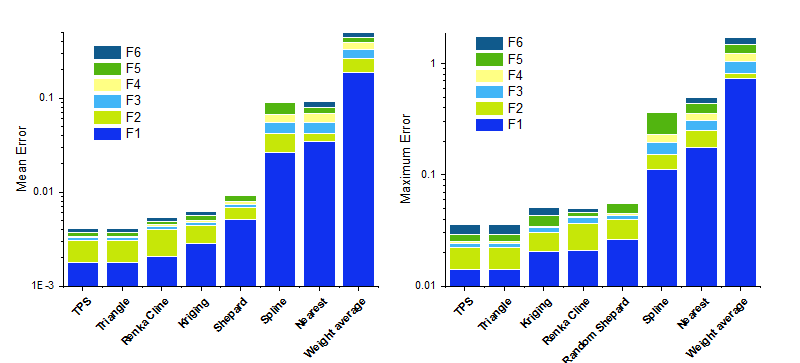
Comparison
Here we offer the comparison of the eight methods. We apply the eight methods to six functions from F1 to F6, which corresponds to exponential peak, cliff surface, saddle surface, gentle peak, steep peak, and sphere surface, respectively. The method is derived from Ref. 2. The interpolation for 1089 points is based on 100 nodes uniform distribution. Mean error and Maximum error are average and max of the difference between real values and interpolated values for 1089 points, respectively. The bar chart for mean error and maximum error are shown below:
Function expression:
^2+(9y-2)^2}{4}}+0.75e^{\frac{-(9x+1)^2}{49}-\frac{9y+1}{10}}+0.5e^{-\frac{(9x-7)^2+(9y-3)^2}{4}}-0.2e^{-(9x-4)^2-(9y-7)^2}")
+1}{9}")
}{6+6(3x-1)^2}")
((x-0.5)^2+(y-0.5)^2)}{3}}")
((x-0.5)^2+(y-0.5)^2)}{3}}")
^2+(y-0.5)^2}}{9}-0.5")
Reference
- Isaaks and Srivastava. An Introduction to Applied Geostatistics, Chapter 12. Oxford University Press (1989)
- R. J. Renka and A. K. Cline. A Triangle-Based
 Interpolation Method, Rocky Mountain Journal of Mathematics. 14, 223-237 (1984) Interpolation Method, Rocky Mountain Journal of Mathematics. 14, 223-237 (1984)
- P. Dierckx. An Algorithm for Surface-Fitting with Spline Functions, IMA Journal of Numerical Analysis. 1, 267-283 (1981)
Related X-Functions
interpxyz
Keywords:interpolate
|