4.3.8 Wavelet

1 Summary
2 What You Will Learn
3 1D Wavelet Transform
4 2D Wavelet Transform
- 4.1 2D Wavelet Decomposition

Summary

Wavelet transforms are useful for analyzing signals which exhibit sudden changes of phase and frequency, local maxima and minima, or related parameters. Wavelet transforms have become a popular tool in time-frequency analysis, especially for analysis of non-stationary signals. OriginPro provides wavelet transform tools for both continuous and discrete transforms.

What You Will Learn

This tutorial will show you how to:

Perform one-level discrete wavelet decomposition and reconstruct a signal from approximation coefficients and detail coefficients.
Apply multi-level discrete wavelet decomposition.
Perform continuous wavelet transform.
Remove noise from signals by using wavelet transform.
Perform 2D wavelet decomposition and reconstruction on matrix data.
Convert an image to matrix data.
Merge graph windows into one graph.

1D Wavelet Transform

Decomposition

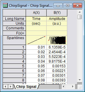
Start with an empty workbook. Select Help: Open Folder: Sample Folder... to open the "Samples" folder. In this folder, open the Signal Processing subfolder and find the file Chirp Signal.dat. Drag-and-drop this file into the empty worksheet to import it.
Highlight column B, and select menu item Analysis: Signal Processing: Wavelet: Decompose... to open the Decompose: dwt dialog.
In the dialog, choose DB6 for Wavelet Type & Order, and Zero-padded for Extension Mode.
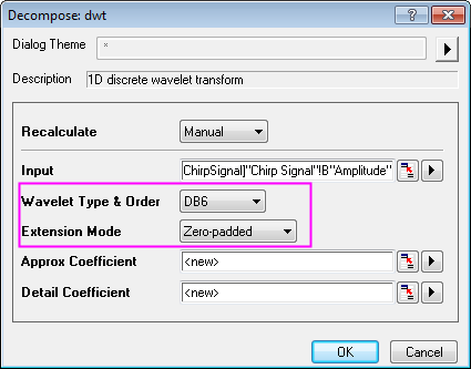
Click OK to close the dialog box and output the approximation coefficients and the detail coefficients.
Highlight columns B, C, and D (columns C and D should contain your approximation coefficients and your detail coefficients, respectively). From the menu, select Plot: Multi-panel: Stack... to open the Stack: plotstack dialog box.
In this dialog, clear the Link Layers check box in the Options node. Check the Auto Preview check box at the bottom to see the preview graph in the right panel.
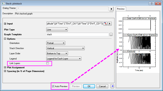
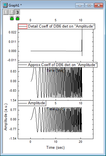
Click OK to close the dialog box and create a stack graph.

Note: To perform level 2 (3, 4, etc.) discrete wavelet decomposition, repeat steps 2 to 4 on the approximation coefficients (column C, in our example). Multi-scale wavelet decomposition (available in OriginPro) is demonstrated below.

Reconstruction

Reconstruction is the inverse operation of decomposition and this example will recover the signal from the result generated above.

Highlight columns C and D (your approximation coefficients and detail coefficients, from above).
Choose menu item Analysis: Signal Processing: Wavelet: Reconstruction... to bring up the Reconstruction: idwt dialog box.
To reconstruct the signal, we need to specify the same Wavelet Type, and Boundary, so set them to DB6 and Zero-padded, respectively.
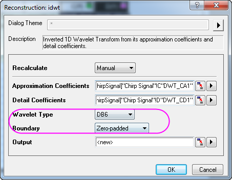
Click OK and the recovered signal is output to column E of the worksheet.
Press CTRL and select columns B and E. From the menu, choose Plot: Line: Line to make a graph with these two columns of data.
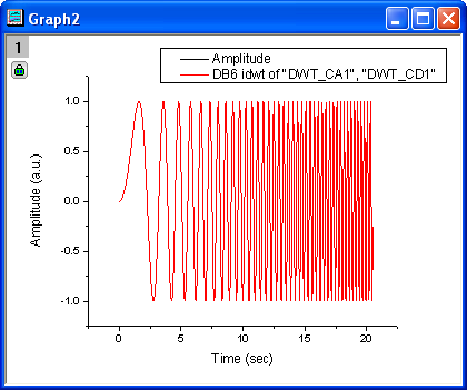
We can see from the resulting graph that the original signal and the recovered signal overlay each other.

Multi-Scale Wavelet Decomposition

Start with a new workbook, and then import the same data used in the Decomposition section above.
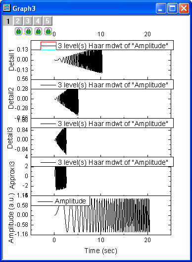
Highlight column B and select menu item Analysis: Signal Processing: Wavelet: Multi-Scale DWT... to open the Multi-Scale DWT: mdwt dialog box.
In the dialog, change Extension Mode to Zero-padded, and Decomposition Level to 3. Click the arrow button beside Multiple Coeff Data and select [<input>]<input> from the menu.
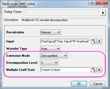
Click OK to obtain 3rd level discrete wavelet decomposition results. The coefficients are stored in the same worksheet as the input signal.
Select all columns in the worksheet, then choose menu Plot: Multi-panel: Stack... to open the Stack: plotstack dialog box. Click the arrow button to the right of Dialog Theme and select System Default. Check the Auto Preview check box at the bottom of the dialog box to preview the graph.
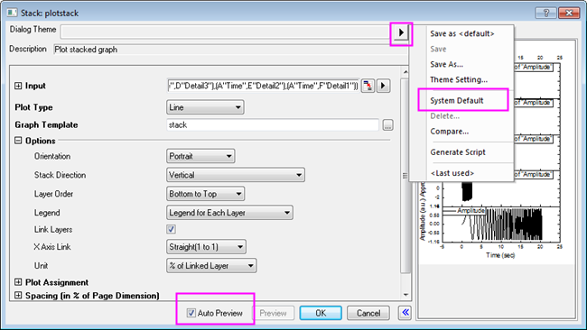
Click OK. The resulting graph is shown below.

Continuous Wavelet Transform

Start with a new workbook with two empty columns (columns A and B) in a single worksheet.
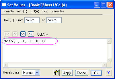
Select column A and then right-click and choose Set Column Values... from the shortcut menu. This opens the Set Values dialog box. In the text box, enter data(0, 1, 1/1023) and click Apply. This fills column A with data.
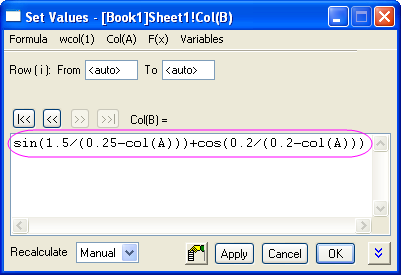
Click the >> button to select column B. Enter sin(1.5/(0.25-col(A)))+cos(0.2/(0.2-col(A))) and click OK.
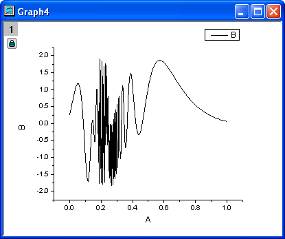
We can make a plot to see how the data looks. With column B selected, choose Plot: Line: Line from the menu.
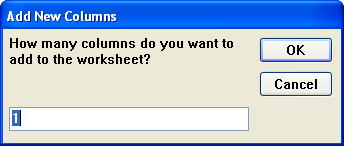
With the worksheet active, add a new column to the worksheet by selecting Column: Add New Columns... from the menu. In the dialog box, accept the default value of 1 and click OK.
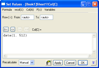
Column C is added to the worksheet. Select it, right-click and choose Set Column Values from the shortcut menu. In the text box, enter data(1, 512) and click OK.
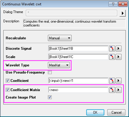
Select both columns B and C, then from the menu, select Analysis: Signal Processing: Wavelet: Continuous Wavelet... to open Continuous Wavelet: cwt dialog box.
In the dialog, set Wavelet Type to MexHat, and check Coefficient Matrix.
Click OK button to exit dialog.
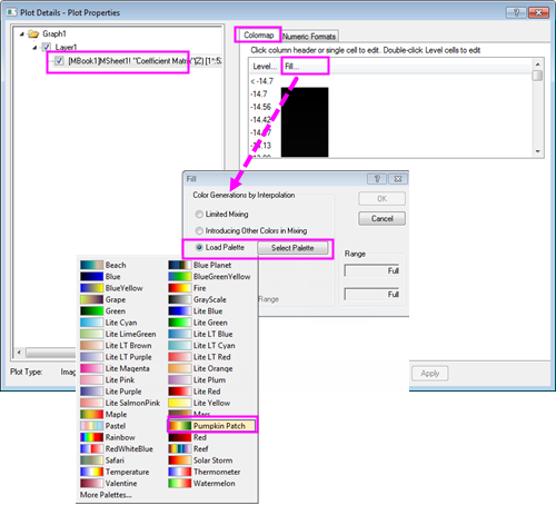
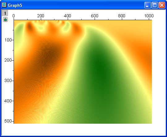
The coefficients are output to a new worksheet and a matrix and a contour plot is added. Double-click on the plot to open the Plot Details dialog box. Select the Colormap tab and click on the Fill... heading. The Fill dialog box opens with color contols. Click Load Palette, and choose Pumpkin Patch from the Select Palette menu. Click OK to return to the Plot Details dialog box.
Click OK to change the color of the contour plot. It should now look like the graph below.

Noise Removal by Wavelet Transform

Start with an empty worksheet. Select Help: Open Folder: Sample Folder... to open the "Samples" folder. In this folder, open the Signal Processing subfolder and find the file Signal with Shot Noise.dat. Drag-and-drop this file into the empty worksheet to import it.
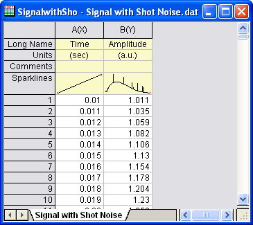
We can see from the Sparklines in the image above that there is shot noise in the signal. Highlight column B and select menu Analysis: Signal Processing: Wavelet: Denoise... to bring up the Denoise: wtdenoise dialog box.
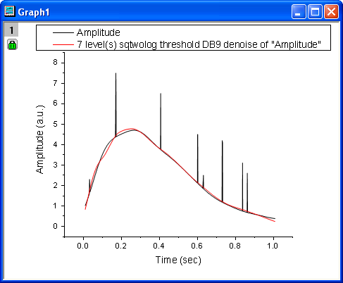
Check Auto Preview to preview your result. Set Wavelet Type to DB9, Extension Mode to Zero-padded, Threshold Type to sqtwolog, and Thresholding Level to 7.
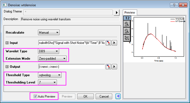
Click OK to remove the shot noise from the signal. Results are output to worksheet columns C and D.
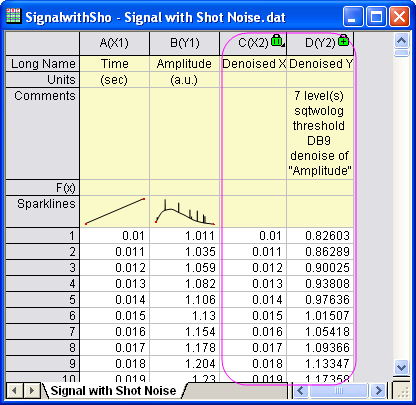
Highlight all columns in the worksheet, then choose menu item Plot: Line: Line to make a graph with the original signal and the cleaned-up signal. We see from the graph below that the shot noise has been removed.

2D Wavelet Transform

2D Wavelet Decomposition

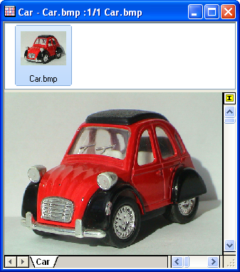
Start with a new matrixbook. From the menu, choose Data: Import from File: Image to Matrix... and import the image, <Origin Installation Directory>\Samples\Image Processing and Analysis\Car.bmp.
To begin, we need to convert the image into data. To do this, select menu item Image: Conversion: Convert to Data. The Convert to Data: img2m opens. Set Type to byte(1).
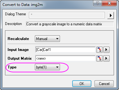
Click OK to obtain the converted matrix data.
With the converted matrix active, select menu Analysis: Signal Processing: Wavelet: 2D Decompose... and open the 2D Decompose: dwt2 dialog box.
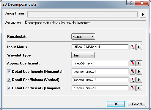
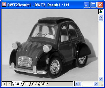
Accept the default settings and click OK. This performs 2D wavelet decomposition on the matrix data. A matrixbook with four matrixsheets (CA, CH, CV, and CD) is generated. CA, CH, CV, and CD contain approximation coefficients, horizontal detail coefficients, vertical detail coefficients, and diagonal detail coefficients respectively. You can change the view mode to image mode by choosing View: Image Mode from the menu.
With the CA matrixsheet active, make an image plot by selecting Plot: Image Plot from the menu. Repeat for CH, CV, and CD matrixsheets.
Double click on graph of them to open the Plot Details dialog, in the left panel, activate Layer1, and then go to the Size/Speed tab in the right panel, and deselect the Matrix data, maximum points per dimension checkboxes. Click OK. select the axes related objects (including axis, label) in the graph and press the DELETE key to delete them.