4.2.2.33 Implicit Fitting with Three VariablesImplicitFit-3Var
Summary
This tutorial will show you how to define an implicit fitting function with three independent variables, then perform implicit fitting with it on fitting data.
Minimum Origin Version Required: OriginPro 9.0 SR1
What you will learn
This tutorial will show you how to:
- Define an implicit fitting function.
- Perform implicit fitting with three independent variables.
- Plot the fitted surface manually.
Examples and Steps
Import Data
- Start with an empty worksheet. Select Help: Open Folder: Sample Folder... to open the "Samples" folder. In this folder, open the Curve Fitting subfolder and find the file Ellipsoid.dat. Drag-and-drop this file into the empty worksheet to import it.
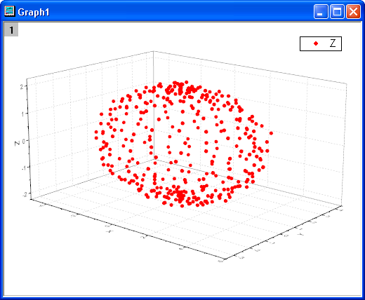
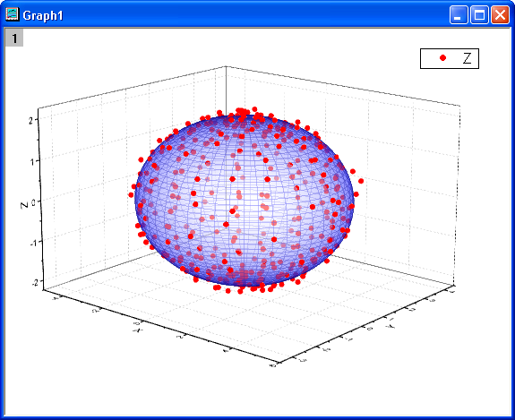
- Highlight column C, right click on selection and choose Set As: Z from the context menu. Select Plot: 3D: 3D Scatter from Origin menu. Double click on the graph. In the Plot Details dialog, select Layer1 in the left panel, click Axis tab, set X, Y, Z Length as 100, 75, 50 respectively. Click the Fit frame to layer button
 in the 3D Rotation toolbar. The graph should look like: in the 3D Rotation toolbar. The graph should look like:
Define Fitting Function
The graph can be fitted with an ellipsoid. The function can be expressed as:
^2}{a^2}+\frac{(y-y_0)^2}{b^2}+\frac{(z-z_0)^2}{c^2}=1")
where  \;") is the ellipsoid's center location, a, b and c are semi-principal axes lengths, x, y and z are three independent variables for fitting data. is the ellipsoid's center location, a, b and c are semi-principal axes lengths, x, y and z are three independent variables for fitting data.
The fitting function can be defined using the Fitting Function Builder tool.
- Select Tools: Fitting Function Builder from the Origin menu.
- In the Fitting Function Builder dialog's Goal page, click Next.
- In the Name and Type page, select Implicit from Select or create a Category drop-down list, type Ellipsoid in the Function Name field, and select Implicit in Function Model group. And click Next.
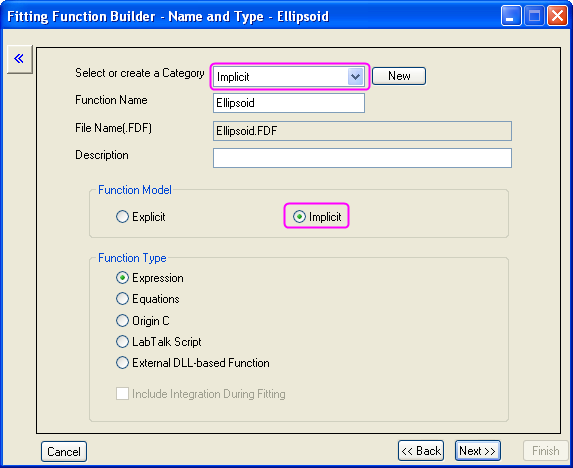
Note that implicit functions must be defined in Implicit category.
- In the Variables and Parameters page, type x, y, z in the Variable field and x0, y0, z0, a, b, c in the Parameter field. Click Next.
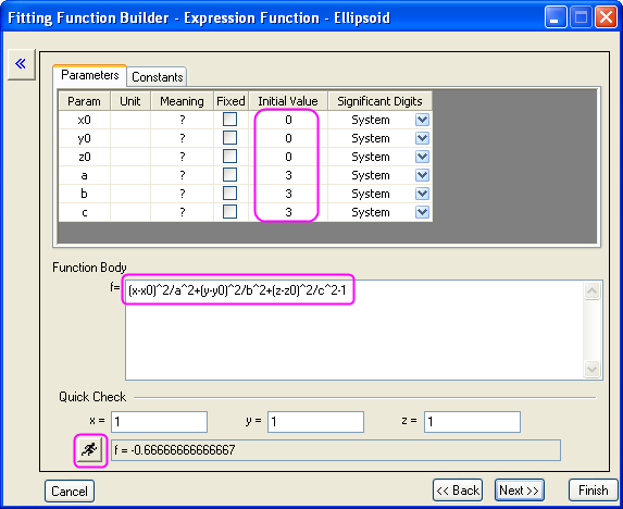
- In the Expression Function page, type the following script in the Function Body edit box.
(x-x0)^2/a^2+(y-y0)^2/b^2+(z-z0)^2/c^2-1 Note that for an implicit function =f_2(x_i,p_i)\;") where where  (i=1,2..) are independent variables, (i=1,2..) are independent variables,  (i=1,2...) are parameters, it must be defined as (i=1,2...) are parameters, it must be defined as -f_2(x_i,p_i)\;") in Origin where f is the Estimate. in Origin where f is the Estimate.
Set initial parameters as follows in the Parameters tab.x0=0 y0=0 z0=0 a=3 b=3 c=3 In the Quick Check group, click Evaluate button, it shows f=-0.667 at x=1, y=1, z=1.
Click Next button, then click Next button again.
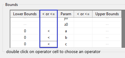
- In the Bounds and General Linear Constraints page, set lower bounds for a, b and c as follows. Then click the Finish button to close the dialog.
-
Note that a message in Messages Log is shown that the implicit function is saved in the User Files folder.
Fit the Curve
- For implicit fitting with more than 2 independent variables, Origin only supports input data from workbooks not graphs. So we have to make the workbook for fitting data active before fitting. Select Analysis: Fitting: Nonlinear Implicit Curve Fit from Origin menu. In the NLFit dialog, select Settings: Function Selection, in the page select Ellipsoid function from the Function drop-down list.
- Select Data Selection page, expand Input Data: Range1, and choose column A as X, column B as Y and column C as Z. An error message is shown at the bottom of the Settings panel. Following the suggestion of the error message, go to the Fitted Curves page and change the Data Type of X to Fitted Point for Input Data. The Data Type of y and z should automatically change as well.
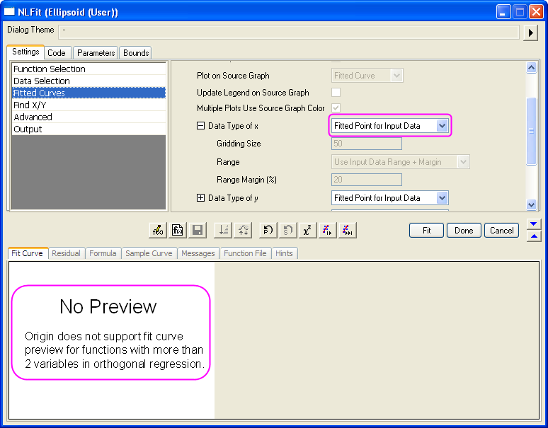
Note that Origin doesn't support Fit Curve preview in the NLFit dialog or fitted surface in the fitted report for implicit fitting with more than two independent variables.
- Since initial parameters have been set in Fitting Function Builder dialog, we can click Fit button to fit the curve.
Fitting Results
Switch to the fitted report. Parameters and Statistics tables are shown in the report.
Fitted Parameters are shown as follows.
| Parameter
|
Value
|
Standard Error
|
| x0
|
0.41073
|
0.01576
|
| y0
|
0.32043
|
0.01352
|
| z0
|
0.00147
|
0.00749
|
| a
|
4.00325
|
0.02076
|
| b
|
3.00097
|
0.01881
|
| c
|
1.99972
|
0.00933
|
And Adj. R-Square is 0.99823, which means the fitted result is very good. Note that this result is from Origin9.0 32Bit, while in Origin9.0 64Bit the result is slightly different, and the latter is better.
In the FitODRCurve1 worksheet, the first three columns show XYY coordinates for fitted points.
Note that in the implicit fitting, x ,y and z are all independent variables, they will all be adjusted during iterations in the fitting.
Fitted Surface
Although Origin9.0SR1 doesn't show the fitted surface in the fitted report for implicit fitting with more than two independent variables, in this example you can plot the fitted ellipsoid using 3D Parametric Function Plot tool in Origin as follows.
- Make the fitted report active, run following LabTalk script in the Script Window in order to get fitted parameter variables.
getnlr tr:=tt;
x0=tt.x0;
y0=tt.y0;
z0=tt.z0;
a=tt.a;
b=tt.b;
c=tt.c;
Variables x0, y0, z0, a, b and c can be used in following steps.
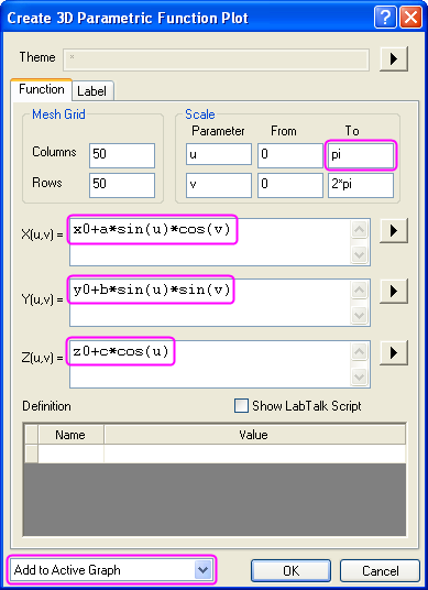
- Make Graph1 active. Select File: New: Function Plot: 3D Parametric Function Plot from Origin menu. In the Create 3D Parametric Function Plot dialog, set u from 0 to pi, v from 0 to 2*pi. And define X ,Y and Z as follows.
X(u,v)=x0+a*sin(u)*cos(v)
Y(u,v)=y0+b*sin(u)*sin(v)
Z(u,v)=z0+c*cos(u)
And choose Add to Active Graph from the drop-down list at the bottom left of the dialog.
Click OK button to close the dialog. A 3D ellipsoid plot will be added to Graph1.
- Double click on the graph. In the Plot Details dialog, you can customize the graph as follows.
Note that only OpenGL of 2.1 or higher version supports 3D transparency in Origin9.0. You can select Preferences: 3D OpenGL Settings from Origin menu to see your OpenGL version, if your OpenGL version is lower than 2.1, you should ignore the setting for 3D transparency in Step 3.2.
- Select Layer1 in the left panel, click Size/Speed tab, clear Worksheet data, maximum points per curve check box in the Speed Mode, Skip Points if needed group. Click Lighting tab, choose Directional in the Mode group, and select blue color as Ambient color in the Light Color group.
- Select the second plot in the Layer1 branch, click Surface tab, set Transparency as 50%. Select Fill tab, and change Fill piece by piece color to white in the Front Surface group. Click OK button to close the dialog.
The graph for the fitted ellipsoid will look like:
|