4.2.2.27 Fitting with Convolution of Two FunctionsFitting-Convolution-2Funcs
Summary
In this tutorial, we will show you how to define a convolution of two functions, and perform a fit of the data with non-evenly spaced X using this fitting function.
 | If your data is a convolution of Gauss and Exponential functions, you can simply use built-in fitting function GaussMod in Peak Functions category to directly fit your data.
|
Minimum Origin Version Required: Origin 9.0 SR0
What you will learn
This tutorial will show you how to:
- Sample a function.
- Calculate a convolution of two functions.
- Define constants in the fitting function.
- Pad zeroes before the convolution.
- Interpolate the convolution result for non-evenly spaced X.
- Use a parameter to balance the speed and the precision.
- Use Y Error Bar as weight.
Example and Steps
Import Data
- Start with an empty workbook. Select Help: Open Folder: Sample Folder... to open the "Samples" folder. In this folder, open the Curve Fitting subfolder and find the file ConvData.dat. Drag-and-drop this file into the empty worksheet to import it. Note that column A is not evenly spaced. We can use LabTalk diff function to verify it.
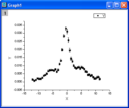
- Right click on column C, and select Set As: Y Error from the short-cut menu. Highlight column B and C, and select Plot: Symbol: Scatter from the Origin menu. The graph should look like:
Define Fitting Function
The fitting function is a convolution of two functions. It can be described as follows:
^2}{w_2^2}}+(f\;*\;g)(x)")
where =\frac{s}{\pi}\cdot\frac{\tau_Lx_0^2(x_L^2-x_0^2)}{(x-x_{c1})\tau_L((x-x_{c1})^2-x_L^2)^2+((x-x_{c1})^2-x_0^2)^2}") , ,
=\frac{1}{w_1\sqrt{\pi/2}}e^{-\frac{2x^2}{w_1^2}}") . .
And  , ,  , ,  , s, , s,  , ,  and and  are fitting parameters. are fitting parameters.  , ,  , ,  , ,  and and  are constants in the fitting function. are constants in the fitting function.
The fitting function can be defined using the Fitting Function Builder tool.
- Select Tools: Fitting Function Builder from Origin menu.
- In the Fitting Function Builder dialog's Goal page, click Next.
- In the Name and Type page, select User Defined from Select or create a Category drop-down list, type convfunc in the Function Name field, and select Origin C in Function Type group. And click Next.
- In the Variables and Parameters page, type x0,xL,tL,s,y0,b1,b2 in the Parameters field, w1,xc1,w2,xc2,A2 in the Constants field. Click Next.
- In the Origin C Fitting Function page, set initial parameters as follows:
x0 = 3.1
xL = 6.3
tL = 0.4
s = 0.14
y0 = 1.95e-3
b1 = 2.28e-5
b2 = 0.2
Click Constants tab, set constants as follows:
w1 = 1.98005
xc1 = -0.30372
w2 = 5.76967
xc2 = 3.57111
A2 = 9.47765e-2
Click the  button on the right of the Function Body edit box and define the fitting function in Code Builder as follows: button on the right of the Function Body edit box and define the fitting function in Code Builder as follows:
Include header files,
#include <ONLSF.H>
#include <fft_utils.h>
Define the function body
  NLFitContext *pCtxt = Project.GetNLFitContext();
  if ( pCtxt )
  {
    // Vector for the output in each iteration.
    static vector vX, vY;

    static int nSize;

    BOOL bIsNewParamValues = pCtxt->IsNewParamValues();

    // If parameters were updated, we will recalculate the convolution result.
    if ( bIsNewParamValues )
    {
      //Sampling Interval
      double dx = 0.05;
      vX.Data(-16.0, 16.0, dx);
      nSize = vX.GetSize();

      vector vF, vG, vTerm1, vTerm2, vDenominator, vBase, vAddBase;

      double Numerator = tL * x0^2 * (xL^2 - x0^2);
      vTerm1 = ( (vX - xc1) * tL * ( (vX - xc1)^2 - xL^2 ) )^2;
      vTerm2 = ( (vX - xc1)^2 - x0^2 )^2;
      vDenominator = vTerm1 + vTerm2;

      //Function f(x)
      vF = (s/pi) * Numerator / vDenominator;

      //Function g(x)
      vG =  1/(w1*sqrt(pi/2))*exp(-2*vX^2/w1^2);

      //Pad zeroes at the end of f and g before convolution
      vector vA(2*nSize-1), vB(2*nSize-1);
      vA.SetSubVector( vF );
      vB.SetSubVector( vG );

      //Perform circular convolution
      int iRet = fft_fft_convolution(2*nSize-1, vA, vB);

      //Truncate the beginning and the end
      vY.SetSize(nSize);
      vA.GetSubVector( vY, floor(nSize/2), nSize + floor(nSize/2)-1 );

      //Baseline
      vBase = (b1*vX + y0);
      vAddBase =  b2 * A2/(w2*sqrt(pi/2))*exp( -2*(vX-xc2)^2/w2^2 );

      //Fitted Y
      vY = dx*vY + vBase + vAddBase;
    }

    //Interpolate y from x for the fitting data on the convolution result.
    ocmath_interpolate( &x, &y, 1, vX, vY, nSize );
  }
Click Compile button to compile the function body. And click the Return to Dialog button.
Click Evaluate button, and it shows y=0.02165 at x =1. And this indicates the defined fitting function is correct. Click Next.
- Click Next. In the Bounds and General Linear Constraints page, set the following bounds:
0 < x0 < 7
0 < xL < 10
0 < tL < 1
0 <= s <= 5
0 < b2 <= 3
Click Finish.
| Note: In order to monitor the the fitted parameters, NLFitContext class was introduced in defining fitting function to achieve some key information within the fitter
|
Fit the Curve
- Select Analysis: Fitting: Nonlinear Curve Fit from the Origin menu. In the NLFit dialog, select Settings: Function Selection, in the page select User Defined from the Category drop-down list and convfunc function from the Function drop-down list. Note that Y Error Bar is shown in the active graph, so column C is used as Y weight, and Instrumental weighting method is chosen by default.
- Click the Fit button to fit the curve.
Fitting Results
The fitted curve should look like:
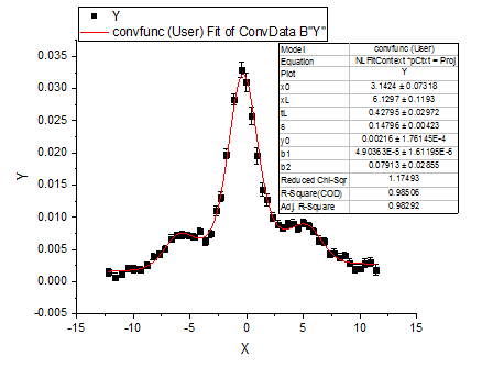
Fitted Parameters are shown as follows:
| Parameter
|
Value
|
Standard Error
|
| x0
|
3.1424
|
0.07318
|
| xL
|
6.1297
|
0.1193
|
| tL
|
0.42795
|
0.02972
|
| s
|
0.14796
|
0.00423
|
| y0
|
0.00216
|
1.76145E-4
|
| b1
|
4.90363E-5
|
1.61195E-5
|
| b2
|
0.07913
|
0.02855
|
Note that you can set a smaller value for dx in the fitting function body, the result may be more accurate, but at the same time it may take a longer time for fitting.
|