4.2.2.15 Fitting with Two Integrals using LabTalk FunctionFitting-2Integral-LabTalk
Summary
In some circumstance, one may want to create fitting function with multiple integrals:
~dt + \int_{LL2}^{UL2} g(x, arg3, arg4, ...)~dx")
We refer to Fitting with Integral using LabTalk Function for detailed description of parameters in the expression.
In version Origin 8.6, however, Fitting Function Builder just supports one integral in fitting function. Bypassing complex Origin C code, we can use Fitting Function Organizer to reach the goal.
In this tutorial, we will show you how to create a fitting function comprised of two integrals using function organizer. Of course, one can include more integrals as desired.
Minimum Origin Version Required: Origin 8.6
 | Beginning with Origin 2018b, you can define a an implicit function using integrals.
|
What you will learn
This tutorial will show you how to:
- Create a fitting function using the Fitting Function Organizer
- Create a fitting function with two integrals using LabTalk function
Example and Steps
The Fitting Model
The fitting model is described as below:
~ dt")
There are four parameters in the fitting function, and we need to pass three of them into the integrand, and use the independent variable as upper limit, to do integration.
Define the Function
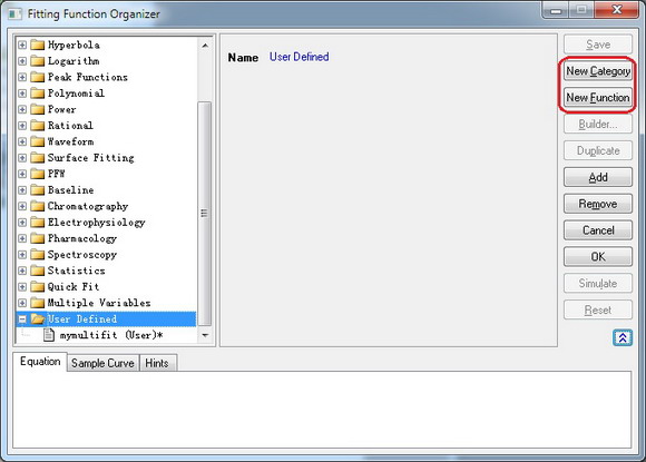
- Press F9 to open Fitting Function Organizer dialog. Add a new function by pressing New Function after you select a category in which you want to put your function. One can also add new category by pressing the New Category button.
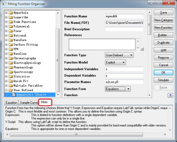
- Specify the function name in the Function Name edit box as you like. Define Independent Variables,
Dependent Variables and Parameter Names in corresponding edit box.
- Select the Function Form in the drop box. One can find explanations in the Hints tab at the bottom of the dialog.
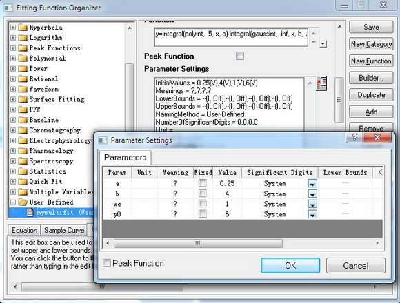
- In the Function edit box, define your fitting function. The integrals are written in the form of LabTalk integral function.
y=integral(polyint, -5, x, a)-integral(gaussint, -inf, x, b, wc)+y0
As described in Fitting with Integral using LabTalk Function, x, a, b and wc are parameters passed into the integrand functions.
- Press the button at the right corner of
Parameter Settings box to active
Parameter Settings dialog. Set initial values as well as other constraints such as lower bounds, upper bounds for each parameter.
- Define the two integrals in the
LabTalk Functions Definition and Initializations box. In this case, the functions should be:
function double polyint(double t, double ia)
{
	return ia*t ;

}


function double gaussint(t, ib, iwc)
{
	return ib *t* exp(-(t)^2/iwc^2) ;
}
- We have successfully set our two integrals fitting function. You can set other information in corresponding box. Do not forget to Save your fitting function after you finish.
Fit the Curve
Copy and paste the following data into Origin worksheet:
| X
|
Y
|
| -3
|
2.47613
|
| -2.6
|
2.24016
|
| -2.2
|
2.01543
|
| -1.8
|
1.83094
|
| -1.5
|
1.85038
|
| -1.1
|
2.17725
|
| -0.9
|
2.44967
|
| -0.7
|
2.61423
|
| -0.5
|
3.02305
|
| -0.3
|
3.23057
|
| -0.1
|
3.37822
|
| 0.1
|
3.2827
|
| 0.3
|
3.18775
|
| 0.5
|
2.86194
|
| 0.7
|
2.69104
|
| 0.9
|
2.39315
|
| 1.4
|
2.04046
|
| 1.8
|
1.85287
|
| 2.2
|
1.85325
|
| 2.6
|
2.20569
|
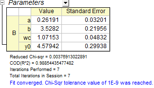
Highlight the Y column, and press Ctrl + Y to open the NLFit dialog. Select the function you just defined, and click fit button  to perform fitting. to perform fitting.
|