5.3.2 One-Way Repeated Measures ANOVA1WayRepeatedMeasuresANOVA
Summary
One-way repeated measures ANOVA is similar to one-way ANOVA, but deals with a dependent variable subjected to repeated measurements. In this situation, the independence assumption of general one-way ANOVA is not tenable, since there is probably a correlation between levels of the repeated factor.
Similar to one-way ANOVA, one-way repeated measures ANOVA can be employed to test whether the means are equal or not. These means include the mean of different measurements and the mean of different subjects. The results will be shown in the table named Test of Within-Subjects Effect and Test of Between-Subjects Effect respectively.
Note that the repeated measures ANOVA in Origin requires balanced sample data, that is, equal sample size at each level.
Minimum Origin Version Required: Origin 8.6 Pro SR0
What you will learn
This tutorial will show you how to:
- Input indexed data iton the statistical analysis dialog.
- Perform One-way Repeated Measures ANOVA.
- Interpret results of a One-way Repeated Measures ANOVA analysis.
Steps
Origin can perform One-Way Repeated Measures ANOVA in both
indexed and raw data mode. For One-Way Repeated Measures ANOVA, if the indexed mode is used, data should be organized into three columns: Factor, data, and Subject. When the Raw data mode
is used, the different levels should be in different columns.
Indexed data mode
The data contains measurements for 3 different doses on 20 subjects, and we are interested in whether different doses on subjects have different effects. To test this, we will perform a One-Way Repeated Measures ANOVA using the indexed data mode.
- Start with an empty worksheet. Select Help: Open Folder: Sample Folder... to open the "Samples" folder. In this folder, open the Statistics subfolder and find the file One Way_RM_ANOVA_indexed.dat. Drag-and-drop this file into the empty worksheet to import it.
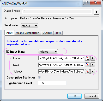
- Select Statistics: ANOVA: One-Way Repeated Measures ANOVA to open the dialog. In the Input tab of this dialog, select Indexed from the Input Data drop-down list and set column B(dose), C(Data), and A(Subject) as the Factor, Data, and Subject respectively.
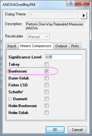
- Go to Means Comparison tab, select the check box after Bonferroni to enable the Bonferroni test.
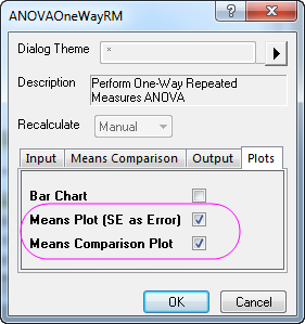
- Select the Means Plot(SE as Error) and Means comparison Plot check boxes in the Plots tab.
- Click the OK button to perform the analysis.
Results Interpretation
Go to the worksheet ANOVAOneWayRM1, where the analysis results are listed.
You can refer to this help file for details of interpreting results of repeated measures ANOVA.
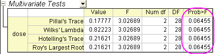
Origin prints out MANOVA automatically alongside repeated measures to detect repeated-measures effects. Note that the four different methods (Pillai's trace, Wilks' lambda, Hotelling's trace, and Roy's largest root) generate identical F statistics and probabilities, P=0.06455, so the means under three levels condition are not statistically different.
Compare with the following report in repeated measures ANOVA, we can see that the conclusion is conservative.

This table shows the results of the Mauchly's Test of Sphericity. From the test results we can see that Sphericity holds. We are interested in the value of Prob > ChiSq, which is the significance level of the Mauchly's Test, we can see from this example that the significance level (0.44609) is greater than 0.05. Therefore, the assumption of Sphericity has not been violated.
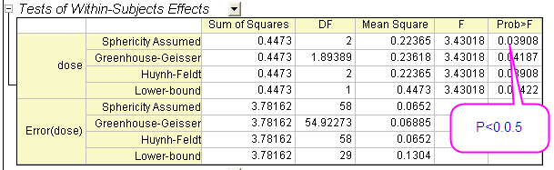
From this table we are able to get the F value for the factor in addition to its associated significance level and effect size. As our data follow the assumption of Sphericity, we can conclude that when using an ANOVA with repeated measures with Sphericity Assumed, the means under three levels condition are statistically different (P = 0.03908 < 0.05). In
other words, dose is a significant factor.
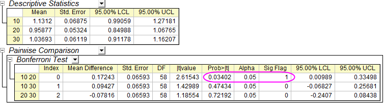
The results presented in the previous table showed that there is an overall significant difference among the means but we do not know where those differences came from. This table shows the results of the Bonferroni test, which allows us to learn which specific means are different. In this case,
the means of dose=10 and dose=20 have a significant difference (P = 0.03402 < 0.05 and Sig Flag = 1).
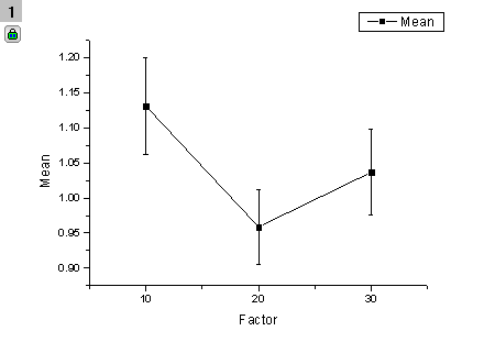
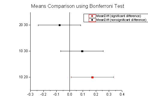
From the two plots below, we can also easily come to the same conclusion.
|