4.2.1.2 Linear Fit for Kinetic ModelsLinear-Fit-For-Kinetic-Models
Summary
Non-linear kinetic models are widely used across many disciplines of natural science, such as, physics, chemistry, biology. Experimentally, all the crucial parameters in kinetic models are obtained through fitting the raw data. The intuitive way to fit the raw data is to do a non-linear fit with the expression directly from the kinetic equation. Alternatively, linear fit can be applied if we can transform the equation in the way that the dependent variable related to independent variable linearly.
Minimum Origin Version Required: Origin 2015
What you will learn
This tutorial will show you how to:
- Perform linear fit on same non-linear kinetic model using different linear transformations.
- Perform apparent linear fit on non-linear kinetic models.
Linear fit for Langmuir model
Identify transformed independent and dependent variables
Langmuir model is described by the non-linear equation below:

where ym, K are the parameters we want to obtain through fitting.
To perform linear fit on Langmuir model, we can transform it into linear equation in two different ways:
- Transform it into traditional linear Langmuir equation:

where the independent variable is y/x, dependent variable is y, slope is -1/K
and intercept is ym.
- Transform it into double reciprocal linear Langmuir equation:

where the independent variable is 1/x, dependent variable is 1/y, slope is 1/(ym*K) and intercept is 1/ym.
Create new independent and dependent variable data
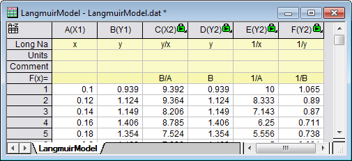
- Open a new workbook. Select Help: Open Folder: Sample Folder... to open the "Samples" folder. In this folder, open the Curve Fitting subfolder and find the file LangmuirModel.dat. Drag-and-drop this file into the empty worksheet to import it.
- If there is a Sparklines label row, right-click it to select Hide from the context menu to hide it. Use Ctrl+D to bring up Add New Columns dialog, enter 4 and click OK to add 4 columns to store transformed XY dataset later.
- For traditional linear Langmuir model transformation, the independent variable is now y/x and dependent variable is still y. Type y/x and y as the long name for column C and D respectively so that it will show as X axis title, Y axis title respectively in later plot.
- Type B/A in F(x) = formula cell in column C to set the value for independent variable y/x, and press ENTER. Highlight column C, right click and select Set As:X to make it as the default X dataset for plotting column D.
- Type B in F(x) = formula cell in column D to set the value for dependent variable y, and press ENTER.
- For double reciprocal linear Langmuir model transformation, the independent variable is 1/x and dependent variable is 1/y. Similarly, make the long name of column E, F as 1/x, 1/y, respectively, and set their column values as 1/A and 1/B accordingly. Set column E designation as X.
- The worksheet is then as following:
Linear fit on transformed linear data
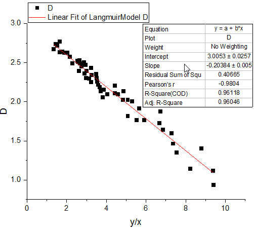
- First, we will perform linear fitting on traditional linear Langmuir transformation. Highlight column D and select Plot:Symbol:Scatter to make a scatter plot.
- To perform linear fitting, select Analysis:Fitting:Linear Fit:Open Dialog to bring up the Linear Fit dialog box and click OK to close dialog. In the appeared prompt, choose No and click OK.
- Similarly, to perform linear fit on double reciprocal linear Langmuir transformation, highlight column F follow the steps above to create a scatter plot and then do a linear fit.
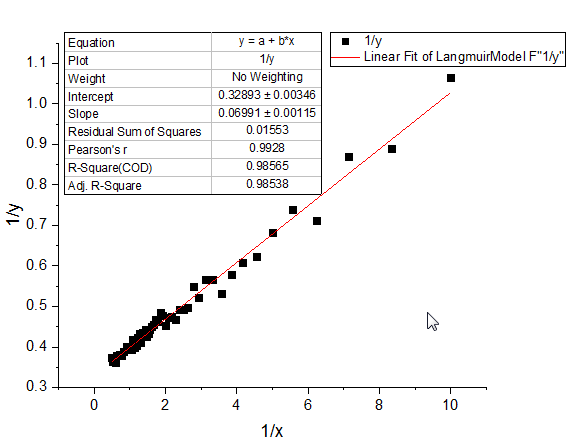
The coefficients in Langmuir model are then can be calculated using corresponding slope and intercept expressions.
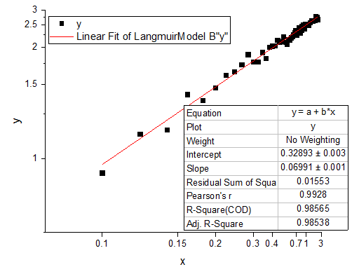
Apparent linear fit on original non-linear data
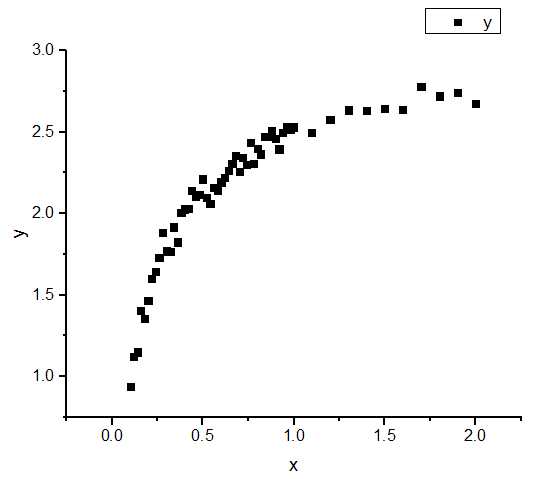
Alternatively, we can use apparent linear fit to directly perform linear fit on raw non-linear kinetic data by customizing only the axis scales. Take Langmuir kinetic model for example, based on double reciprocal Langmuir linear transformation we found that the inverse of original dependent variable 1/y is in linear relationship with the inverse of original independent variable 1/x. Therefore, if set the X scale as 1/x and set the Y scale as 1/y, raw Langmuir kinetic data would appear with linearity.
- To perform apparent linear fit on Langmuir kinetic raw data, highlight column B and select Plot:Symbol:Scatter to make a non-linear scatter plot.
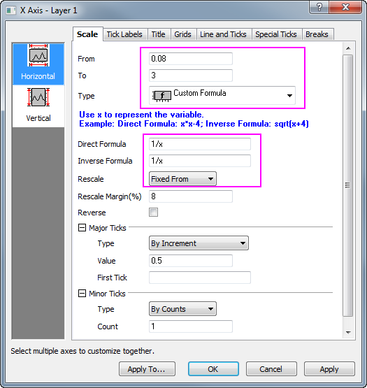
- Double click on the X axis to bring up Axis dialog, set From as 0.08 and To as 3. Then select Custom Formula from the Type drop-down list and input 1/x as the Direct Formula and 1/x as the Inverse Formula. Choose Fixed From in the Rescale drop-down list. Click OK to close the dialog.
- As can be see from the plot, the default X axis ticks are not well separated. To make the ticks of X axis display reasonably, we will create a dataset to set the positions of ticks. To do so, activate LangmuirModel worksheet and use Ctrl+D to add one more column. Enter dataset 0.1, 0.15, 0.2, 0.3, 0.4, 0.7, 1, 3 in newly added column G.
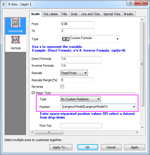
- To use column G as major tick positions for X axis, double click on the X axis to bring up Axis dialog. Then go to Major Ticks node choose By Custom Positions from Type drop-down list and choose [LangmuirModel]LangmuirModel!G from the Dataset drop-down list.
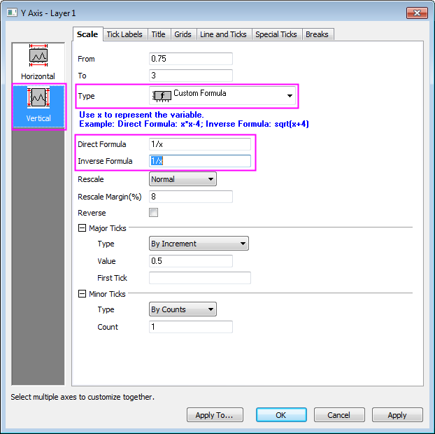
- Click Vertical icon on left panel, similarly, choose Custom Formula from Type drop-down list and input 1/x in both Direct Formula and Inverse Formula boxes. Click OK to close the dialog box.
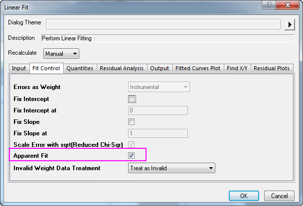
- To perform apparent linear fit, select Analysis:Fitting:Linear Fit:Open Dialog to bring up the Linear Fit dialog box. In the Fit Control tab, we can see that by default the Apparent Fit box is checked.
- Click OK to close dialog and choose No radio box in the prompt, then click OK to close it.
Solutions for other non-linear kinetic models
Freudlich equation
The non-linear kinetic equation for Freudlich model is as below:
 = ln(K)+\frac{ln(x)}{n}")
where the independent variable is ln(x), dependent variable is ln(y), slope is 1/n and intercept is ln(K), K and n are the coefficients to be determined.
Apparent linear fit is recommended since Ln scale is a build-in scale setting. To fit this non-linear kinetic model, use apparent fit with X and Y axis scales both set to be Ln scales.
Alternatively, you can perform linear fit after you calculate the Ln value of both X and Y dataset. See the example of Langmuir model above for details.
Lagergren's pseudo-first order
The non-linear kinetic equation for Lagergren's pseudo-first oder model is as below:
 = \frac{log(q_{e,fit})-k_1*x}{2.303}")
where the independent variable is x, dependent variable is ") , slope is , slope is  and intercept is and intercept is /2.303") , ,  is known constant, is known constant,  and and  are the coefficients to be determined. are the coefficients to be determined.
Apparent linear fit is recommended since Log scale is a build-in scale setting. To fit this non-linear kinetic model, first calculate  and then use apparent fit with only Y axis scale set to be Log scale. and then use apparent fit with only Y axis scale set to be Log scale.
Alternatively, you can firstly calculate ") and use this newly created data to do linear fit directly. Refer to the example of Langmuir model above for details. and use this newly created data to do linear fit directly. Refer to the example of Langmuir model above for details.
Ho's pseudo-second order
The non-linear kinetic equation for Freudlich model is as below:

where the independent variable is x, dependent variable is x/y, slope is  and intercept is and intercept is ") , ,  and and  are the coefficients to be determined. are the coefficients to be determined.
To linearly fit this model, you have to firstly calculate x/y and use this newly created data to perform linear fit.
Alternatively, we can transform this equation into the form below:

where the independent variable is 1/x, dependent variable is 1/y, slope is and intercept is .
For this transformation, we can either perform linear fit once we created new independent variable data as 1/x and new dependent variable data as 1/y. Or we can perform apparent linear fit by set both X and Y axis scales as 1/x scale. Please refer to Langmuir model for more details.
|