5.3.4 Two Way Repeated Measures ANOVA

2WayRepeatedMeasuresANOVA

Summary

For Two-Way Repeated Measures ANOVA, "Two-way" means that there are two factors in the experiment, for example, different treatments and different conditions. "Repeated-measures" means that the same subject received more than one treatment and/or more than one condition. Similar to two-way ANOVA, two-way repeated measures ANOVA can be employed to test for significant differences between the factor level means within a factor and for interactions between factors. Using a standard ANOVA in this case is not appropriate because it fails to model the correlation between the repeated measures, and the data violates the ANOVA assumption of independence. Two-Way Repeated Measures ANOVA designs can be two repeated measures factors, or one repeated measures factor and one non-repeated factor. If any repeated factor is present, then the repeated measures ANOVA should be used.

In the following example, the two factors are the repeated measures factors.

Minimum Origin Version Required: Origin 8.6 Pro SR0

What you will learn

This tutorial will show you how to:

• Input raw data in the statistical analysis dialog.
• Perform Two-Way Repeated Measures ANOVA.
• Interpret results of a Two-Way Repeated Measures ANOVA

Steps

Origin can perform Two Way Repeated Measures ANOVA in both indexed and raw data modes. For Two-Way repeated measures ANOVA, if the indexed mode is used, data should be organized into four columns: Factor A, Factor B, Data, and Subject. When the Raw data mode is used, the different factors and levels should be in different columns.

In this example, we are interested in whether different drugs and doses have different effects on subject. We will perform the Two-Way Repeated Measures ANOVA to determined whether the drug type and dosage have significant effect on a subject. If there is significant difference, we will perform pairwise comparison to determine of which level the effects are different.

Raw data mode

1. Start with an empty worksheet. Select Help: Open Folder: Sample Folder... to open the "Samples" folder. In this folder, open the Statistics\ANOVA subfolder and find the file Two-Way_RM_ANOVA_raw.dat. Drag-and-drop this file into the empty worksheet to import it.
2. Select Statistics: ANOVA: Two-Way Repeated Measures ANOVA to open the dialog.
3. In Input tab, select Raw from the Input Data drop-down list.
4. In this example, there are two factors. Set 3 and 2 for Number of Levels in Factor A and Factor B drop-down list to specify levels of the factor. Set Name to drug and dose respectively.

5. Now under the Data branch, there are three subgroups. In the drug Level1 subgroup, select column d1d1 as the dose Level1 input data range.
6. Similarly, select d1d2, d2d1, d2d2, d3d1, and d3d2 for the next 5 input data range.
7. Check the Interactions check box to calculate interaction effects.
   
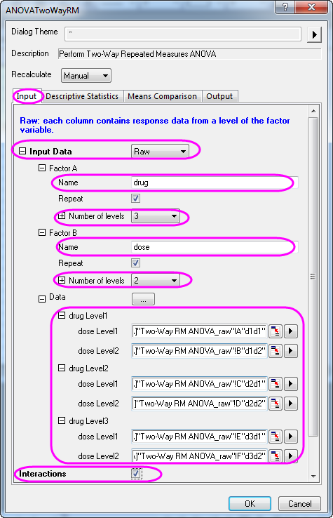
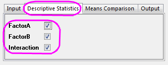
8. In the Descriptive Statistics tab, select all check boxes to compute the mean, standard error, and 95% confidence interval of all the levels of the factors as well as interactions.
   
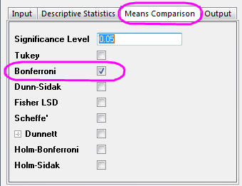
9. In the Means Comparison tab, select the Bonferroni check box to enable the Bonferroni test.
   
10. Click the OK button to perform the analysis.
    

Results Interpretation

Go to the worksheet ANOVATwoWayRM1, where the analysis results are listed.

You can refer to this help file for details of interpreting results of repeated measures ANOVA.

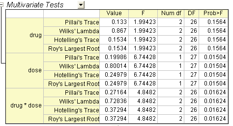
Origin uses a multivariate analysis to detect repeated-measures effects. In this example, four different methods (Pillai's trace, Wilks' lambda, Hotelling's trace, and Roy's largest root) generate identical F statistics and probabilities. For drugs, P_value=0.1564, so we can conclude that the effect of drugs did not reach conventional levels of statistical significance. Similarly, we can also conclude that dose and drugs* dose are significant.

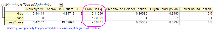
This table shows the results of Mauchly's Test of Sphericity and evaluation of epsilon. From the column Prob>ChiSq, we can learn that the significance level of drugs is greater than 0.05 (P_value=0.11096), and the value of drugs*dose is smaller than 0.05. For drugs*dose, the assumption of sphericity has been violated. Note that Greenhouse-Geisser Epilon=0.65362, which is smaller than 0.75, so we will proceed with the test by using Greenhouse-Geisser correction.

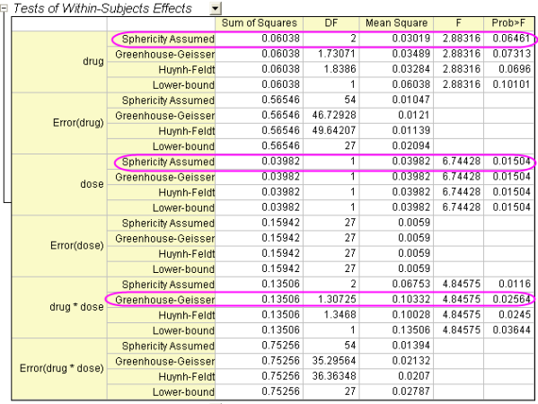
From this table we are able to find out the F value for the factor, its associated significance level and the effect size. For drug, the P_value is 0.06461 in the prob>F column, so drugs have no significant effect on subjects, while dose have(P_value=0.01504). For interaction drugs*dose, we can still proceed with the test by using the Greenhouse-Geisser correction and conclude that interaction drugs*dose have significant effect (P_value = 0.02564).

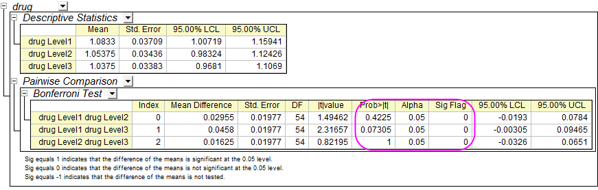
In general, Bonferroni tests are recommended to determine which specific means differed and determine whether or not the Sphericity assumption is violated. The Bonferroni correction relies on a general probability inequality and therefore isn't dependent on specific ANOVA assumptions. This table presents the results of the Bonferroni test, we can conclude that the means are not significant different (P>0.05 and Sig Flag=0). Of course, we do not need to perform pairwise comparison because drugs have no significant effect.

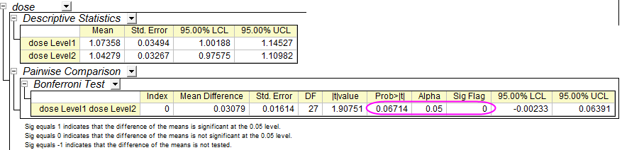
In this table, we can conclude that means of different dose are not significantly different (P_value = 0.06714 and Sig Flag = 0).

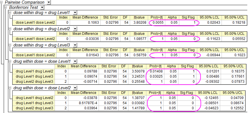
In this table, we can conclude that dose1 is significantly larger than dose2 within drug1, and drug1 is significantly larger than drug2 and drug3 within dose1.