5.8.4 Partial Least Squares

Partial-Least-Squares

Summary

Partial least squares (PLS) is a method for constructing predictive models when there are many highly collinear factors.

This tutorial will start with the spectral data of some samples to determine the amounts of three compounds present. The data includes:

• Data of the spectra emission intensities at different wavelength (v1 - v43)
• Amount of the three compounds in the sample (comp1, comp2, comp3)

This tutorial will establish a model to predict the amount of the three compounds from v1 - v43

Minimum Origin Version Required: OriginPro 2016 SR0

Partial Least Squares Regression

1. Start with a new project or a new workbook. Import the data file: \Samples\Statistics\MixtureSpectra.dat
2. Highlight Column("v1") through Column("v43").
3. Select Statistics: Multivariate Analysis: Partial Least Squares. This opens the pls dialog box to the Input Data tab.
4. The highlighted columns are automatically added as independent variables. Click the triangle button next to Independent Variables, and click Select Columns... in the context menu.
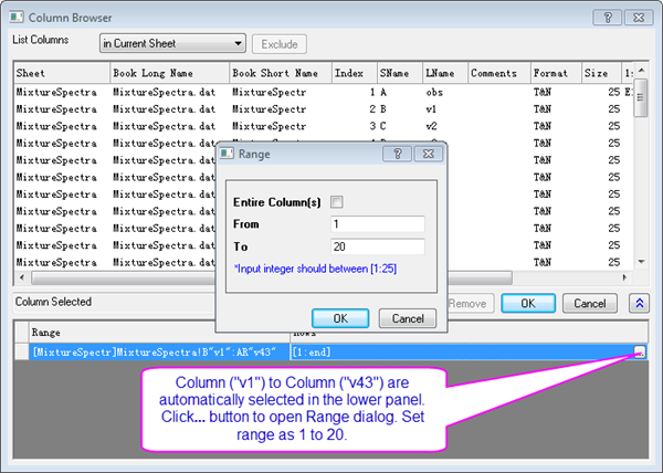
5. Ensure the lower panel is expanded by clicking the button with two arrows in the bottom right of the Column Browser dialog.
6. In the lower panel click the ... button. A Range dialog box will open. Clear the Entire Column(s) box and set the data range from 1 to 20. Click OK, then click OK to close the Column Browser.

   

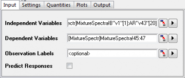
7. Click the interactive button to the right of Dependent Variables. Return to the worksheet, select column("comp1") and drag to column("comp3"). Click the interactive button again to restore the dialog box.

   

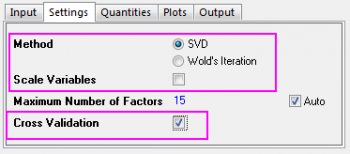
8. Since v1 to v43 are absorbance, there is no need to standardize them. Click on the Settings tab, set Method to SVD and clear the Scale Variables check box.
9. Select the Cross Validation check box. It helps find the optimal number of factors in the model.

   

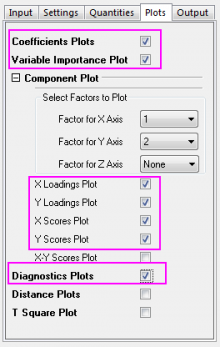
10. Click the Plots tab and expand the Component Plot branch. Select the following check boxes and click the OK button.
    • Variable Importance Plot
    • X Loadings Plot
    • Y Loadings Plot
    • X Scores Plot
    • Y Scores Plot
    • Diagnostics Plots

Developing the Model

In the workbook, select the tab for the PLS1 sheet:

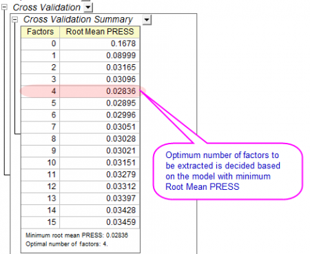
1. The Cross Validation table shows the optimum number of factors to extract. PRESS is the predicted residual sum of squares of the model. The model with minimum Root Mean PRESS has the optimal number of factors:

   

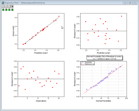
2. The Diagnostics Plots are residual plots of Y and X, which can be used to judge the quality of the model. Overall we can say that the fitted model is good because:
   • Layer 1 - The Predicted values-Actual values graph indicates that the model fits well for the first component.
   • Layer 2 - In the Predicted values-Residual graph, residuals are randomly distributed around zero. This indicates that there is no drift in the process.
   • Layer 4 - The P-P plot of residual can be used to check whether the variance is normally distributed. The result falls almost in a line, which means the variance is normally distributed.

   

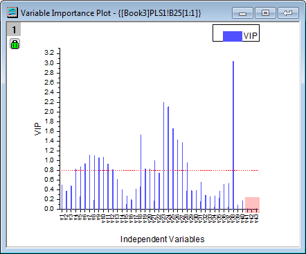
3. A summary of importance of v1~v43 is given by the VIP plot. If the variable has small regression coefficients and low VIP values, we can consider excluding it in the model. For example
   • VIP values of v41 ~ v43 in the plot below are low:

     

   • Coefficients of v41 ~ v43 are also small in the three coefficients below:

     

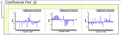
   However, as in step 2, it appears that the model fits well so it is also acceptable to keep these less important variables.

Interpreting the Results

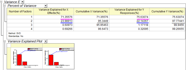
1. The Variance Explained table shows the proportion of variance explained by each factor. In the example, Factor 1 explains 71.36% variance for the X effect and 75.6% variance for the Y effect. Factor 2 explains 23.99% variance for the X effect and 22.14% for the Y effect. The Variance Explained Plot indicates that more attention should be paid to the first two factors as these two explained more than 95% variance for X and Y effects.

   

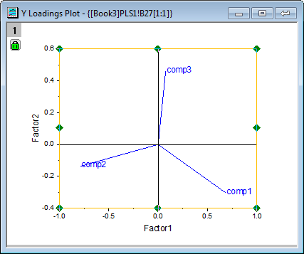
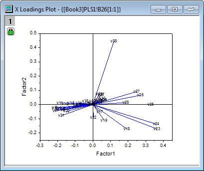
2. The Loading Plot reveals the relationships between X and Y variables in the space of the first two factors.
   • From the Y loading plot we can see that the three compounds have different loading on Factor 1 and Factor 2.

     

   • From the X loading plot it is apparent that v26 ~ v38 have similar heavy loadings for Factor 2, and v17, v18, v19,v23 and v24 have similar light loadings for factor 1 and factor 2.

     

Notes: To examine the plot in detail, you can double-click to open the graph containing the loading plot and zoom in it with the Scale In tool

Using the Model to Predict

After the model is established, we can predict the amounts of the three compounds in new samples from their spectra emission intensities at different wavelengths:

1. Click the green lock on the PLS1 sheet and select Change Parameter from the context menu.
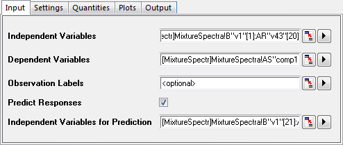
2. In the dialog that opens, click on the Input tab and select the Predict Responses check box.
3. Click the interactive button to the right of Independent Variables for Prediction. Return to the workbook, select the MixtureSpectra sheet. Select column("v1") to column("v43"). Click the interactive button again to restore the dialog box.
4. Click the triangle button next to Independent Variables for Prediction, and then click Select Columns... in the context menu.
5. In the lower panel of the Column Browser dialog, click the ... button. Deselect the Entire Column(s) box and set the data range from 21 to 25. Click OK to close the Range dialog and Column Browser dialog..

   

6. Click the OK button to apply the settings and close the dialog.
7. The PLSResults1 sheet will now contain the predicted amounts of the three compounds in the five new samples:
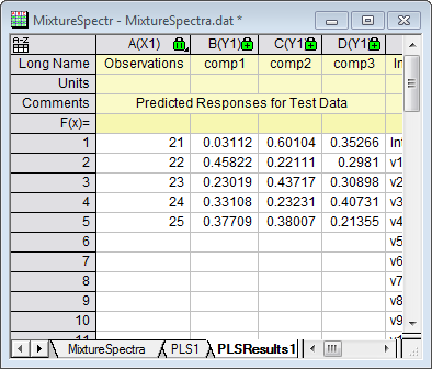