5.9 Power and Sample SizePower-SampleSize
Summary
Power and sample size analysis is useful in design of experiments. Insufficient data translates into a lack of power to reject a false null hypothesis and collecting too much data is a waste of time and resources. Therefore, it is essential to determine the sample size requirements prior to conducting an experiment. The power of the experiment can be computed for a given sample size, and required sample sizes can be computed for given power values.
What you will learn
This tutorial will show you how to calculate sample size or estimate power value to design experiments, using some practical examples.
(PSS)One-Sample t-Test
Background:
A sociologist wants to determine whether the average infant mortality rate in the United States is equal to 8. In experiment design, the difference of rate cannot vary more than 0.5. And it is already known that the standard deviation should be 2.1 from pilot studies.
Question:
What would the sample size be, in order to estimate the average infant mortality rate at a confidence level of 95% ( =0.05) for power values of 0.7, 0.8 and 0.9? =0.05) for power values of 0.7, 0.8 and 0.9?
Steps in Origin:
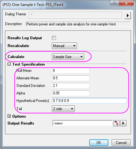
- Activate an empty worksheet, select Statistics: Power and Sample Size: (PSS) One-sample t-test;
- In the PSS_tTest1 dialog box, choose the following settings and click OK.
Origin Output:
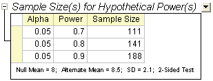
A result sheet will be generated, listing the calculated sample size for hypothetical powers.
Result Interpretation:
According to results, when designing his experiment the sociologist should conduct a survey of 111 samples for a power value of 0.7; 141 samples for power value of 0.8; and 188 samples for power value of 0.9.
(PSS)Two-Sample t-Test
Background:
A doctor's office participates in two local insurance plans, Healthwise and Medcare. The purpose is to compare the mean time (in days) until reimbursement of claims for the two plans. Historical data shows that for the Healthwise plan, the average time is 32 days and the standard deviation is 7.5 days. For the Medcare plan, the average reimbursement time is 42 days and the standard deviation is 3.5 days.
Question:
If 10 claims from each plan were selected and the corresponding reimbursement times were recorded, what is the power to detect the difference in mean reimbursement times between the 2 plans by 5% or more?
Steps in Origin:
- Compute the pooled standard deviation as:
^{*}7.5^{\land} 2+(5-1)^{*}3.5^{\land }2)/(5+5-2)}=5.85235")
*Note that this value will be used as the standard deviation later for the power calculation.
- Sample size of 1st group and 2nd group should be 10 (20 samples total).
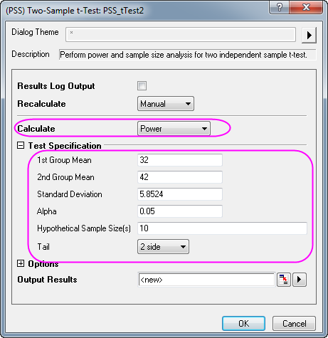
- Activate an empty worksheet and select Statistics: Power and Sample Size: (PSS) Two-Sample t-Test,
- In the PSS_tTest2 dialog box, choose the following settings and click OK.
Origin Output:
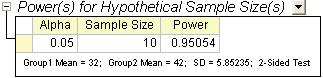
A result sheet will be generated, showing the calculated power.
Interpretation of Results:
We can conclude that the doctor's office has a 0.95054:1 (or 95%) chance of detecting a difference if it collects 10 claims for each plan. The chance that you will fail to reject the null hypothesis and incorrectly conclude that the two means are not different is 4.946% (1 - 0.95054).
(PSS)Paired-Sample t-Test
Background:
Two machines of the same type are used to measure the depth of an amorphous silicon (a-Si) thin film. To determine if there is a difference in the two machines measurements, an engineer plans a study to compare the depth measurements made by the two machines.
In a previous study on depth of the a-Si thin film, the standard deviation of the difference was found to be 2µm. In addition, it is known that the difference in measurement by the two machines should not exceed 0.5µm, and the average depth measured by Machine #1 is 5000µm.
Question:
How many samples must be taken at a confidence level of 99% to obtain power values of 0.8, 0.9 and 0.95?
Steps in Origin:
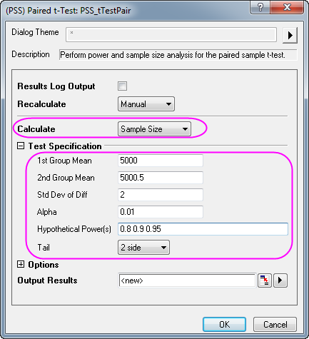
From the information above, it is concluded that the mean of the 1st group is 5000 µm and the mean of the 2nd group is 5000.5 µm.
- Activate an empty worksheet and select Statistics: Power and Sample Size: (PSS) Paired t-Test
- In the PSS_tTestPair dialog box, set controls as in the following image and click OK.
Origin Output:
A result sheet will be generated, listing the required sample size at different power values.
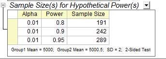
Interpretation of Results:
We conclude that the engineer has an 80% chance of detecting a difference if 191 thin film samples are measured; a 90% chance if 242 thin film samples are measured; and a 95% chance if 289 thin film samples are measured by each machine.
(PSS)One-Way ANOVA
Background:
Researchers are interested in whether different plants have different nitrogen contents. They planned to record nitrogen contents in milligrams for 4 species of plants (80 observations per species). Previous research suggests that the square root of MSE (Mean Squared Error) is 60 and the CSS (corrected sum of squares) of the means is 400.
Question:
Is the plan feasible? (i.e. will the calculated power be acceptable?)
Steps in Origin:
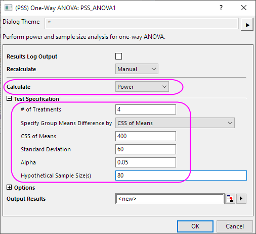
- The sample size for each group is 80.
- Activate an empty worksheet and select Statistics: Power and Sample Size: (PSS)One Way ANOVA
- In the PSS_ANOVA1 dialog box, choose the following settings and click OK.
Origin Output:
A result sheet is generated, and the power value is calculated from the known condition.
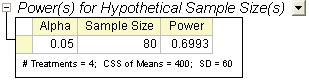
Interpretation of Results:
It appears that the original research plan is deficient. There is only a 69% chance of detecting a difference from each group. To get more reliable results, researchers must collect more samples per species of plant.
|