5.2 Hypothesis TestsHypothesis-Tests
Summary
Hypothesis tests are frequently used to measure the quality of sample parameters or to test whether estimations for two samples on a given parameter are equal .
With parametric methods,assumptions are made about the underlying distribution from where the sample populations are selected. Usually, it requires that the data are independently sampled from a normal distribution.
What you will learn
This tutorial will show you:
- How to carry out hypothesis tests for practical data with Origin
- How to interpret the generated results
Steps
Hypothesis Tests in Origin
| Data Type
|
Goal
|
Method
|
| One Sample
|
Compare the mean with a given value
|
One-Sample t-Test
|
|
|
Compare the variance with a given value
|
One-Sample Test for Variance
|
| Two Samples
|
Test whether the means are equal
|
Two-Sample t-Test
|
|
|
Test whether the variance are equal
|
Two Sample Test for Variances
|
| Paired Samples
|
Test whether the means are equal
|
Pair-Sample t-Test
|
One-Sample t-Test
Perform One-Sample t-Test using Raw data
Suppose a manufacturer produces high-quality screw nuts that must equal 21 millimeters in diameter. The quality control department randomly drew 120 nuts from the finished products, measured the diameters for each and stored the results in Diameters.dat file. They want to determine whether the mean diameter of the nuts is equal to 21 or not. Historically, the distribution of the measured diameters is known to be approximately normal, but the standard deviation of the population is unknown. Hence they may use the One-Sample t-Test in Origin following the steps below:
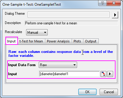
- Start with a new workbook and import the file \Samples\Statistics\diameter.dat.
- Open the One-Sample t-Test dialog by using the menu item Statistics:Hypothesis Testing:One-Sample t-Test.
- Click the Input tab, set Input Data Form to Raw.
- Click the arrow button to the right of Input and select A(X):diameter.
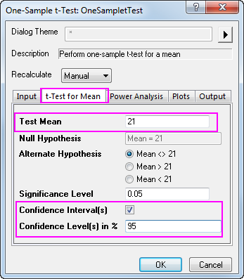
- Click the t-Test for Mean tab and set Test Mean to 21; Make sure that Alternate Hypothesis is set to Mean <> 21 (two-sided test), check Confidence Interval(s) and set Confidence Level(s) in % to 95.
- Note that by default the test procedure provides descriptive statistics of the variable and the hypothesis test results. Additionally, it is possible to produce a histogram of the data and a confidence interval for the mean.
- Click the OK button to finish the analysis and generate results.
The Descriptive Statistics table shows the sample size, mean, standard deviation, and standard error for the variable. The sample mean, 21.00459, is comparatively little bigger than the hypothesis mean 21, and the standard error of the mean(SEM) is 0.00156.
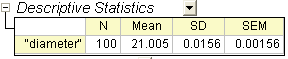
From the t-Test table, the t statistic (2.9437) and the associated p-value (0.00404) provide evidence that the average diameter of screw nuts is significantly different with 21 at the  level. level.
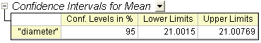
The confidence interval indicates that it is 95% confident that the true mean of the variable lies within the interval [21.0015, 21.00769].
Perform One-Sample t-Test using Summarized data
To perform a One-Sample t-Test using summarized data, we need to change the Input Data From in Input tab into Summarized data.
Assume we have measured 70 nuts this time, so the sample size will be 70. After a further calculation, we have got 20.95 for the mean, and 0.218 for the standard deviation. So we enter the mean, standard deviation and sample size into the Input Box below:
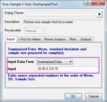
Then, we set 21 as the Test Mean in t-Test for Mean tab, click OK to execute.
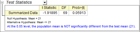
We get the summary table shown below, the results indicate that the population mean is NOT significantly different from the test mean in this study.
Pair-sample t-Test
Perform Pair-sample t-Test using Raw data
Suppose you want to compare abrasion resistance between two kinds of tires. You randomly draw from each type of tires respectively and group them into 8 pairs. Make sure each pair consists of two types of tires. Next, equip the paired tires on 8 planes to run the abrasion test and measure the abrasion data to do paired-sample t-test.
- Start with a new workbook and import the file \Samples\Statistics\abrasion_raw.dat.
- Open the Pair-sample t-Test dialog by using the menu item Statistics:Hypothesis Testing:Pair-sample t-Test.
- On the Input tab, set column tireA as 1st Data Range and column tireB as 2nd Data Range.
- Click the t-Test for Mean tab and enter 0 to be Test Mean.
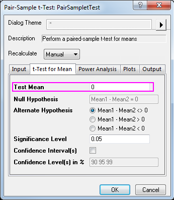
- Accept other settings as default and click the OK button to generate results.
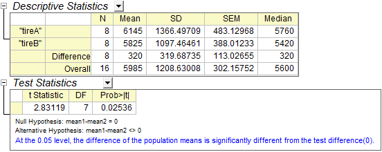
From the t-Test table, the t statistic (2.83119) and the associated p-value (0.02536) indicate that the difference between the two means is significant, that is to say, the two types of tires have different abrasion resistance.
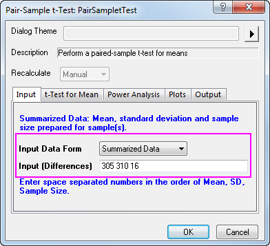
Perform Pair-sample t-Test using Summarized data
Perform Pair-Sample t-Test using Summarized data
To perform a Pair-Sample t-Test using summarized data, we need to change the Input Data From in Input tab into Summarized data.
Assume 16 samples has been tested this time, so the sample size will be 16. After a further calculation, we have got 305 for the mean paired difference, and 310 for the standard deviation for the difference between paired data points (please refer to Algorithms: Pair Sample T-Test). So we enter the mean difference, standard deviation and sample size into the Input Box below:
Since our data yielded a p-value of 0.0013, which is less than our 0.05 a-level, we can reject the null hypothesis.
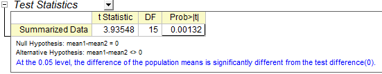
This study indicates the difference between the two means is significant, thus, the two types of tires have different abrasion resistance.
Two-Sample independent t-Test
Perform Two-Sample t-Test using Raw data
A physician is evaluating the effect of two kinds of soporifics. To test the effectiveness of these two medicines, 20 insomniacs patients are randomly selected. Half took medicine A and the other half took medicine B, The extended sleeping time were recorded after each patient took the medicine. The result is saved as the time_raw.dat file.
To determine whether the two medicine have different effect on patients, we could carry out a two-sample independent t-test with the following steps:
- Start with a new workbook and import the file \Samples\Statistics\time_raw.dat.
- Open the Two-Sample t-Test dialog by using the menu item Statistics:Hypothesis Testing:Two-Sample t-Test.
- On the Input tab, select Raw for the Input Data Form; set medicineA as 1st Data Range and medicineB as the 2nd Data Range.
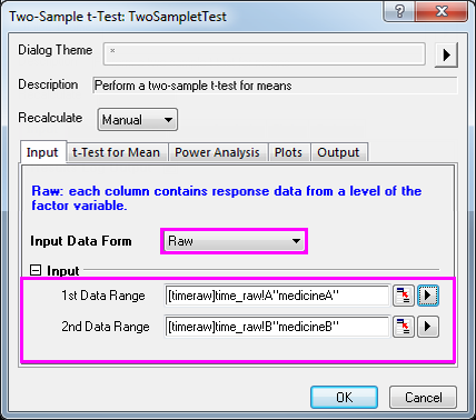
- Accept other settings as default and click the OK button to generate results.
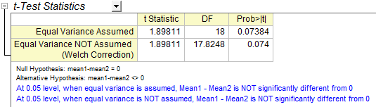
The t-Test procedure automatically provides two tests of the mean difference. One is based on the assumption that the variances of two samples are equal and the other is not. In this example, both tests indicate that there is no significant evidence for a difference in cure effects between medicine A and medicine B. (p-values are 0.0738 and 0.074, both greater than the significance level 0.05.)
Perform Two-Sample t-Test using Summarized data
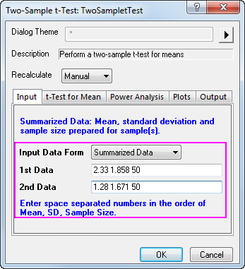
To perform a Two-Sample t-Test using summarized data, we need to change the Input Data From in Input tab into Summarized data.
Assume 50 patients has been tested this time, so the sample size will be 50. After a further calculation, we have got 2.33 for the 1st mean, and 1.858 for the 1st standard deviation, and 1.28 for the 2nd mean, and 1.671 for the 2nd standard deviation. So we enter the mean, standard deviation and sample size into the Input Box below.
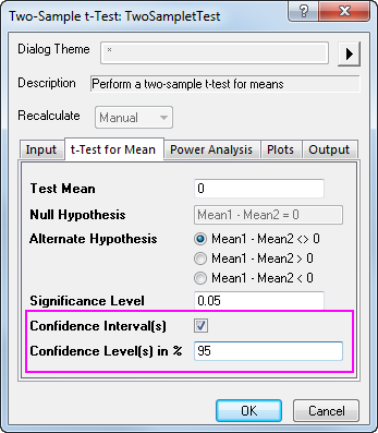
We can also check on the Confidence Intervals (Levels in 95%) in t-Test for mean tab, to calculate the difference between test groups. Click OK to execute.
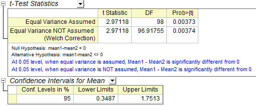
Since our data yielded a p-value of 0.0037, which is less than our 0.05 a-level, we can reject the null hypothesis. this study indicates that the mean extended sleeping of two patients groups are not the same. In fact, we can conclude that 1st soporific has a stronger effect on patients.
The Confidence Intervals show that we can be 95% confident that the mean time difference between two groups is 0.3487~1.7513
 | Note that both equal variance and unequal variance assumptions are supported.To determine whether the two samples have equal variances, we may select from top menu Statistics:Hypothesis Testing:Two-Sample Test for Variance to use the two-sample test for variance for testing
|
Two-Sample Test for Variance
- Continue with a new workbook and import the file \Samples\Statistics\time_raw.dat.
- Open the Two-Sample Test for Variance dialog by using the menu item Statistics:Hypothesis Testing:Two-Sample Test for Variance.
- Select "Raw" for the Input Data Form; set column A and column B as the first and second data range respectively.
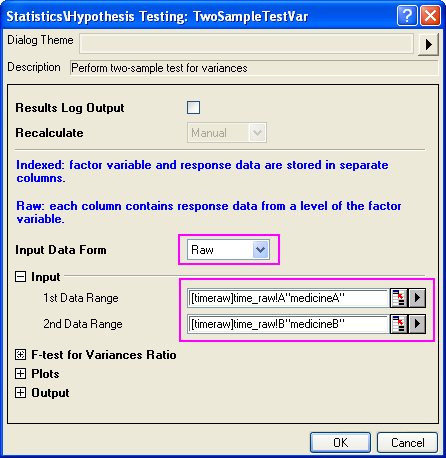
- Accept other settings as default and click the OK button to generate results.
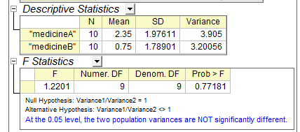
According to result , P_vaule=0.77181 >0.05,therefore ,it fail to reject null hypothesis, so two population variances are not signification difference.
|