The Origin workbook is a nameable, moveable, sizeable window that provides a framework for importing, organizing, analyzing, transforming, plotting and presenting your data.
|
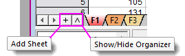
Two convenient buttons were recently added to the workbook window: Add Sheet and Show/Hide Organizer. |
| Object | Maximum Number |
|---|---|
|
Worksheets in a workbook |
1024† |
† > 255 sheets requires saving file to Unicode-compliant (e.g. *.opju) file format. Unicode formats not compatible with Origin versions prior to Origin 2018.
| Workbooks |
|
|---|---|
| Worksheets |
|
| Columns |
|
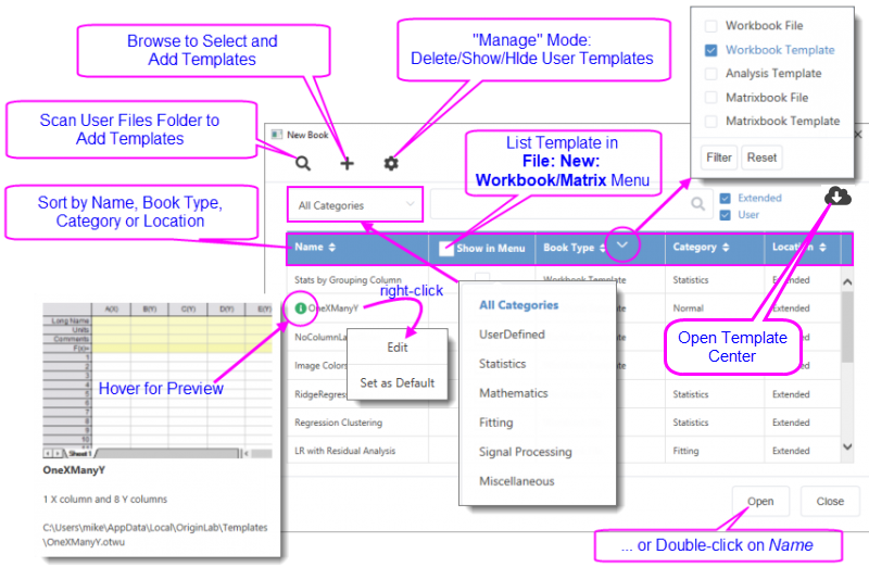
Origin workbooks are highly customizable and can be saved with data (e.g. Workbook File) or without data (e.g. Workbook Template). Since they can be configured for many different applications, there is a good chance that you will collect a number of custom files over time. The New Book dialog is useful for organizing and choosing these files for use.
or
|
An Open Template Center button |
|
Each window's Properties dialog has a Comments box for entering text. These comments are included in the New Book dialog previews and the Project Explorer previews. In addition, comments are searchable from the Edit: Find in Project tool. |
Origin workbooks support Spreadsheet Cell Notation (SCN). Spreadsheet Cell Notation allows the sort of cell-level calculations that are familiar to users of spreadsheets (more details below).
The workbook serves as a flexible container for all of your work-related data -- not just text and numeric data. You can add graphs, matrices, images, notes; and store calculations, scripts and variables, text objects and programmable buttons, and create live links to other project data. Beyond its role as a flexible data container, the workbook can also serve as a medium for batch analysis and reporting.
This table summarizes the kinds of objects that can be saved in the workbook window at the workbook, worksheet and worksheet cell levels, and how to access them.
| Element | Workbook | Worksheet | Worksheet Cell |
|---|---|---|---|
| Graphs | Right-click on the sheet tab > Add Graph as Sheet | Right-click in the gray area beyond the last column > Add Graph | Right-click on the cell > Insert Graph |
| Matrices | Right-click on the sheet tab > Add Matrix as Sheet | -- | -- |
| Images | -- | -- | Right-click on the cell > Insert Images from Files |
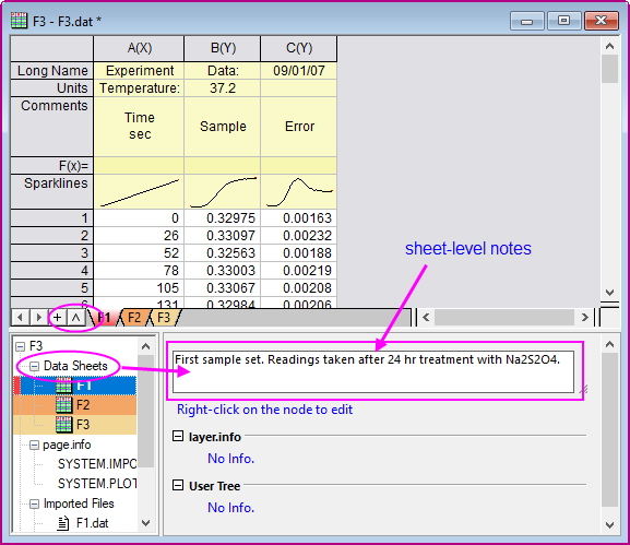
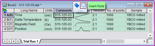
| Notes | Right-click on workbook title bar > Properties > Comments | Click the workbook's Show/Hide Organizer button > Data Sheets > enter notes in box | Click on the cell and Insert Note with the Mini Toolbar (see below). |
| Variables | Click the workbook's Show/Hide Organizer button > page.info, Imported Files, User Tree, etc. | Added text objects linked to data/variables | Right-click on the worksheet cell and Insert Variables; or select a cell and Define Name using Mini Toolbar. |
| Functions and Formulas | Right-click in the gray area to the right of last column > Show Script Panel | Select a column, right-click and Set Column Values. Alternately, enter formula in F(x)= cell. | Click on a cell and use the Formula Bar or direct cell entry, to create cell formula. |
| Scripts | Right-click in the gray area to the right of last column > Show Script Panel |
|
-- |
| File Metadata | Click the Show/Hide Organizer button on the workbook toolbar | -- | -- |
| Links | -- | -- | Enter cell-level links to URLs, other worksheet ranges/cells, project graphs, matrices and image files. |
| Text and Drawing Objects | -- | Add Programmable Buttons and Text Labels and Drawing Objects to the worksheet. | -- |
| Arrows | -- | -- | Right-click and Insert Arrow |
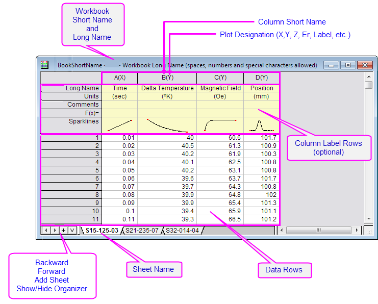
A workbook can have up to 1,024 sheets. A sheet has a single Name which can contain spaces and special characters. Optionally, you can add a Label and/or a Comment.
To edit the sheet Name
System variable @SSL can be used to modify sheet naming behavior. Look for @SSL in the LabTalk System Variable List.
|
When mousing over the worksheet tab, Name, Label and Comments appear as a tooltip. |
To add worksheets to the workbook, right-click on a worksheet's tab and choose one of the following:
Each sheet in a workbook can have its own set of customizations. When you Insert or Add a worksheet, the new sheet is based on the ORIGIN.otwu file (specifically the version of ORIGIN.otwu that is saved to your User Files Folder if you have customized this file). To add a sheet that is based on another sheet in the workbook (including number of columns and special formatting), you would use the Duplicate or Duplicate Without Data shortcut command.
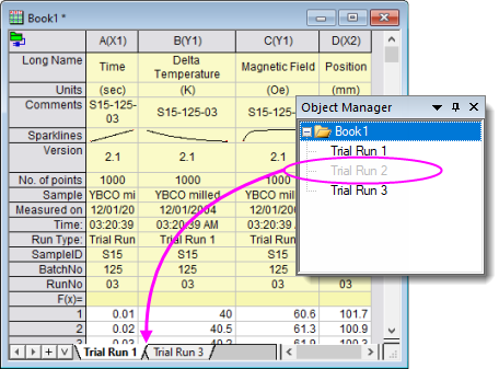
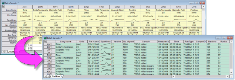
To move sheets between existing books or use them to create new books:
You can also (a) drag existing sheets between books or (b) drag and drop sheets onto an empty portion of the workspace, to create a new book.
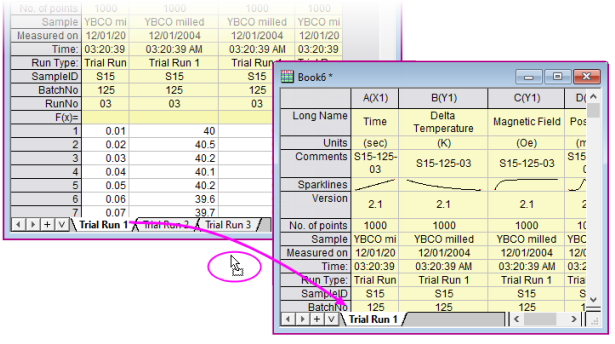
To select multiple sheets when dragging between books or when dropping sheets onto the workspace to create new books:
or...
To open the Worksheet Properties dialog
You can use the Worksheet Properties dialog box to customize properties of the sheet, including...
Note that many of the sheet customizations can be applied at the cell level by right-clicking on a selected cell and choosing Format Cells.
For more information, see The Worksheet Properties dialog box.
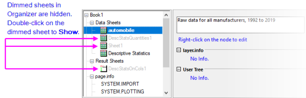
Use the Object Manager's shortcut menu commands to manipulate display of workbook content:
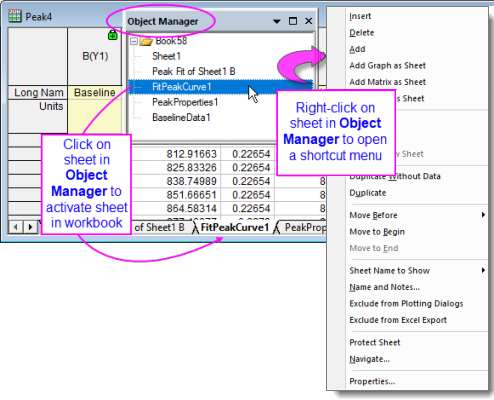
You can hide (and show) worksheets by using the Object Manager.
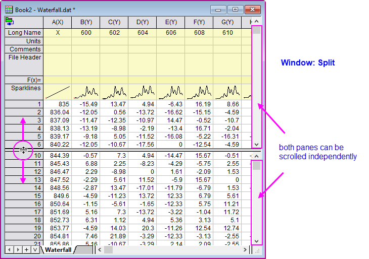
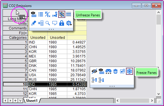
Origin has two utilities for locking the view in part of the worksheet, while allowing you to scroll through the remainder of the sheet. The two could be used interchangeably in some situations.
This places a moveable, vertical or horizontal divider at the selected row or column; or if a single cell is selected, both a vertical and a horizontal divider. This divides the worksheet into identical and scrollable views of the worksheet data area. The user is able to scroll within each panel while rows or columns in the other panel(s) remain visible.
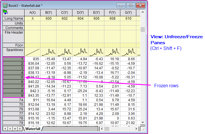
The user can freeze the first 1 to 10 rows and/or columns in the worksheet, thus locking them in view while the remainder of the rows or columns remain scrollable. Locked row and column headers are shaded in a darker color to indicate freeze.
Worksheet columns can be renamed by:
See the above table for rules on worksheet column naming.
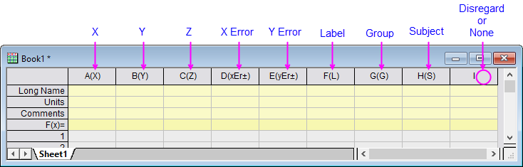
As mentioned, worksheet Column Designations (aka "Plot Designations") generally determine how data are handled during analysis and plotting operations. For instance, you might select an X column + three Y columns to perform a simultaneous linear fitting of each Y dataset against a common set of X values. Or you might select the same columns to graph 3 line plots against a common set of X values. In addition, there are designations for Z values, for error data, for labels, etc. (for more information, see Setting Column Designation in the Origin Help file).
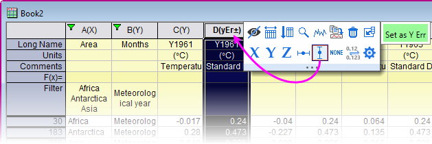
While there are a number of places in the user-interface where you can designate columns during some analysis or plotting operation, at a basic level, they are set in the worksheet by (1) clicking on the column header to select a column, then (2) doing one of the following:
The Column Properties dialog box is used to customize properties of the column including...
To open the '''Column Properties''' dialog box:
Use the Properties tab to edit the column Short Name, if desired. Other properties -- Long Name, Units and Comments -- can be edited here or entered directly into the column label row cells.
Data in the Origin worksheet is treated as either text or numeric data. While the display of text data in the worksheet is fairly straightforward, the display of numeric data is more complicated.
Unless otherwise specified, all numbers in the worksheet are stored internally as floating point, double precision (Double(8)) numbers. This includes date and time, data which is formatted to display in degrees-minutes-seconds or numbers that are formatted to display a fixed number of decimal digits.
When dealing with numeric data, understand that what you see in the worksheet is a representation of a number that is stored internally. This is important for two reasons:
|
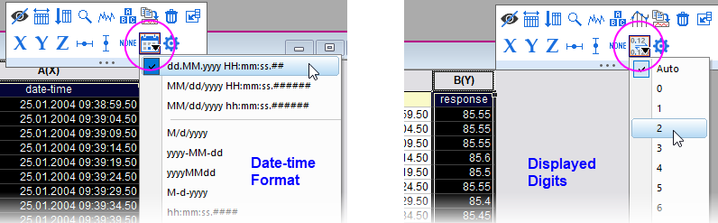
While the central place for formatting worksheet data is the Properties dialog, as described above, keep in mind that there are quick-access Mini Toolbar buttons for changing the Display of numeric and date-time data. Note that the Format of selected columns must first be set as Date or Numeric/Text & Numeric for these buttons to be visible.
|
By default, Origin stores date-time data as a modified Julian Day value and it uses this number for date-time calculations. Typically, however, you will prefer to display this Julian Day value in a more meaningful date-time format:
|
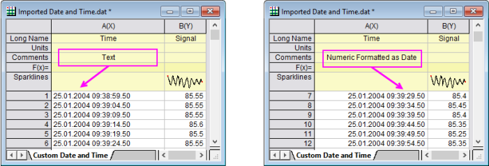
When importing date-time data into the worksheet, Origin will sometimes treat this data as text (Origin's CSV Connector generally does a better job of recognizing date-time data). If your date-time data are left-aligned in the worksheet cell, Origin "sees" it as text. You will need to open the Column Properties dialog box and choose your Format and Display options. When you see that your date-time data are right-aligned in the cell, you know that Origin "sees" the data as numeric data, displaying in a date-time format. |
Origin 2021 introduced a new column and cell Format -- Color.
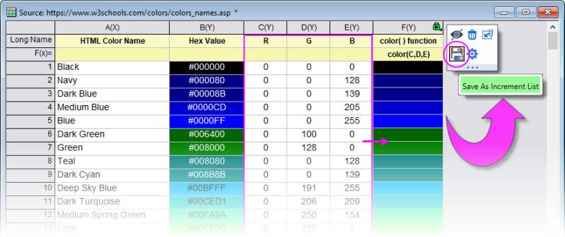
color(A,B,C) sets color using RGB values in columns A, B and C).
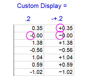
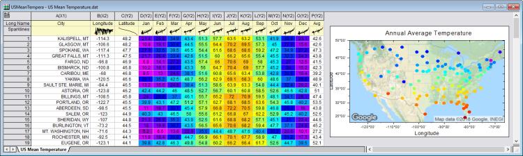
Origin can display numeric values in the worksheet in a variety of custom formats. This illustration shows various formats applied to the same set of numeric values (column A(X)).
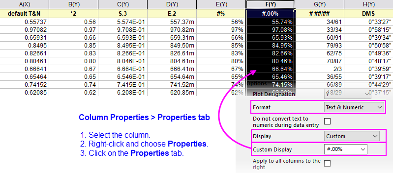
The following is a sample listing of some supported custom format options (this just happens to be the pre-populated list that ships with Origin 2019). Note that you can enter custom formats directly into the Custom Display list and they will be saved to this list.
There are many other format options. For more information, see Custom Numeric Formats
| Format | Description | Example if cell value = 123.456 |
|---|---|---|
| *n | Display n significant digits. | *3 displays 123 |
| .n | Display n decimal places. | .4 displays 123.4560 |
| S.n | Display n decimal places, in scientific notation of the form 1E3. | S.4 displays 1.23456E+02 |
| E.n | Display n decimal places, in engineering format. | E.2 displays 123.46 |
| * "pi" | Display a number as a decimal, followed by the symbol π. | * "pi" displays 39.29727π |
| #/4 "pi" | Display a number as a fraction of π, with a denominator of "4". | #/4 "pi" displays 157π/4 |
| #/# "pi" | Display a number as a fraction of π. | #/# "pi" displays 275π/7 |
| ##+## | Display a number as two digits, a "+" separator, then two digits (e.g. surveying stations). | ##+## displays 01+23 |
| #+##M | Display a number as one digit, a "+" separator, then two digits, plus a suffix of "M". | #+##M displays 1+23M |
| #n | Display a number as an integer of n digits, pad with leading zeros as needed. | #5 displays 00123 |
| #% | Display a number as a percentage. | #% displays 12346% |
| # ##/## | Display a number as proper fraction. | # ##/## displays 123 26/57 |
| # #/n | Display a number as proper fraction, in nths. | # #/8 displays 123 4/8 |
| DMS | Display a number in Degree° Minute' Second", where 1 degree = 60 minutes, and 1 minute = 60 seconds. | DMS displays 123°27'22" |
| D MDn EW (longitude) D MDn NS (latitude) |
Display a number in Degrees and Decimal Minutes. Parameter n specifies decimal places. Positive values will have "E" or "N" appended, Negative values will have "W" or "S" appended. If you wish to preserve negative values do not append "EW" or "NS". | D MD3 EW displays 123° 27.360 E |
| D MDn EWB (longitude) D MDn NSB (latitude) |
Display a number in Degrees and Decimal Minutes. Parameter n specifies decimal places. Letter "B" ("before") specifies that positive values should have "E" or "N" prefixed, negative values will have "W" or "S" prefixed. If you wish to preserve negative values do not append "EWB" or "NSB". | D MD3 EWB displays E 123° 27.360 |
| %#x | Display a number as a 32-bit hexadecimal (max 8 hexdigits). The "#" symbol specifies "Ox" prefix. | %#x displays 0x7b |
| %#0nx | Display a number as a 32-bit hexadecimal (max 8 hexdigits) notation, as an n-character string, pad with leading 0 as needed. | %#06x returns 0x007b |
| %#0nI64X | Display a number as a 64-bit hexadecimal notation (max 13 hexdigits, 15 total including #="0x"), as an n-character string, pad with leading 0 as needed. | %#014I64X returns 0X00000000007B |
| -+n |
Display a negative/positive (-+) format that can be combined with other custom formats. For instance, if you had a column containing both positive and negative numbers, you might set Custom Display as "-+.2" to display numbers to 2 decimals with a prefix of "-" or "+". Normally (by default), the "-" does display while the "+" does not. However, this syntax also substitutes a "long minus" in place of the usual "short minus" used in displaying worksheet negative numbers. Note that the "-" and "+" symbols may be combined in your custom string (e.g. "-+") or used alone (e.g. "-").
|
-+.2 displays +123.4560 |
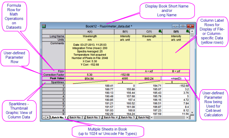
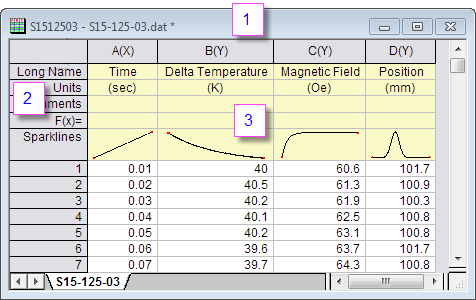
Column label rows store metadata -- data that is used to describe other data. Typically, this metadata may be brought in as header information in imported files, or it may be manually entered. Display of column label rows is optional and the user can selectively show them or hide them, as needed.
Column label row information is often used in plotting operations (e.g. worksheet Long Names used as graph legend text or Axis titles). The F(x)= row is used in performing math operations on columns of data (see below). Data stored in User-defined Parameter rows might be used in labeling or grouping of datasets in plotting, data manipulation, statistical analysis or math operations (see Tutorial 2, below).
Tips...
Display (showing or hiding) of column label rows is controlled by shortcut menu commands:
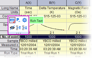
There is also a worksheet column label row Mini Toolbar for managing label rows. Use it to do such things as hide selected label rows, enable Rich Text or change label row order.
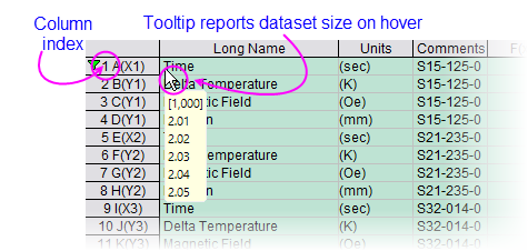
Origin 2019 introduced a new view mode for the worksheet called Column List View that is a transposed view of the column label row metadata. This view is potentially useful if your worksheets have many rows of metadata and you want to focus on some particular aspect of that metadata. With the worksheet active, choose View: Column List View or press Ctrl + W.
Further, you can apply a data filter to metadata in Column List View. When you return to the standard worksheet view (clear the mark beside View: Column List View), only data associated with the filtered metadata will show in the worksheet.
|
Column List View displays column index number ahead of column short name (+ column designation). In addition, you can hover on the left edge of column long name and a tooltip reports dataset size. To disable the display of column index, set @DSI=1. |
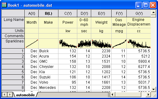
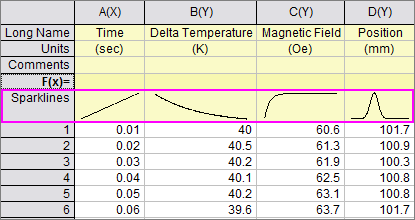
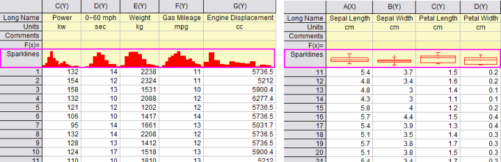
Numeric data stored in a column will graphically display in the column header in a special label row called Sparklines. A sparkline is, by default, a small inset line plot of the data in a column, plotted as the dependent variable (Y) against the row number or the associated X column as independent variable (X). When importing data, Origin displays sparklines by default when the number of columns is less than 50.
To Show or Hide Sparklines:
|
Sparklines can, in large numbers, cause Origin to act sluggishly. If your project is difficult to work with and you suspect sparklines may be contributing, you can prevent sparkline creation and hide existing sparklines in the project using system variable @SPK. Additionally, you can delete sparklines from the current project using delete -spk. |
As mentioned, the workbook commonly stores metadata, some of which is visible in the column label rows. Other metadata may be hidden in the workbook. Such hidden metadata might include things like import file path and name, date and time of data import, file header information not written to the column label rows, variable names and values, etc. This hidden metadata can be viewed in the Workbook Organizer panel.
To show (or hide) a workbook's Organizer panel:
A number of common book-, sheet-, column and cell-level properties can be set or toggled ON/OFF with a Mini Toolbar button.
|
Origin has another "Replace" tool that can be scripted: wreplace. To open a UI dialog, open the Script Window (Window: Script Window) and type wreplace -d. To learn about scripting options, see the X-Function documentation for wreplace. |
Origin provides several utilities for filling a worksheet range or column, with data. The simplest of these use a menu command to fill a worksheet column with either row index numbers, uniform random numbers or normal random numbers. This is useful for generating quick datasets to test and try out other Origin features.
These simple procedures create a dataset in a pre-selected worksheet range or column(s):
| Action | Toolbar Button | Menu Command |
|---|---|---|
| Fill a range or column with row numbers |
or
|
|
| Fill a column with uniformly distributed random numbers between 0 and 1 |
or
|
|
| Fill a column with normally distributed random numbers |
or
|
|
| Fill a column with a patterned or random set of numbers | -- |
|
| Fill a column with a patterned or random set of Date/Time Values | -- |
|
| Fill a column with arbitrary set of Text&Numeric values | -- |
|
The auto fill feature can be used in filling column label rows and the worksheet data cells:
To use auto fill to extend a pattern in the data across a range of cells (numeric data only):
To use auto fill to repeat a pattern in the data across a range of cells (text or numeric data):
|
Tips of data selection methods:
|
Datasets can also be generated quickly using LabTalk script. As an example:
col(1)={0:0.01:4*pi};
col(2)=sin(col(1));
The Set Values dialog box is used to set up a mathematical expression that creates or transforms one or more columns of worksheet data. The dialog box includes a menu bar, a control used to define output range, a tool for searching and inserting LabTalk functions into your expression, a column formula box used to define a one-line mathematical expressions, a Before Formula Scripts panel (usage optional) intended for data pre-processing and defining of variables used in your one-line expression and for Python users, a Python Function tab for defining and using Python functions which can also be used in your expressions.
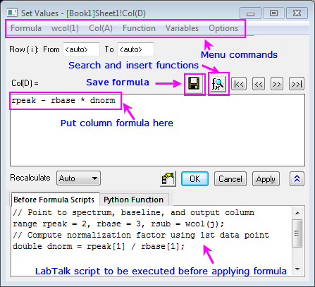
Since Origin 2017, the column formula box (the upper box) in Set Values has supported a simplified spreadsheet cell notation like is used in MS Excel and Google Sheets. A cell is addressed using column Short Name + row index number (e.g. the first cell in column A -- formerly represented as "col(A)[1]" -- is now simply "A1").
In new workbooks, spreadsheet cell notation is enabled by default. Spreadsheet cell notation can only be used in defining the column formula. It cannot be used in the Before Formula Scripts panel of Set Values, nor can it be used in your LabTalk scripts. Note that the "old" column and cell notation will work in spreadsheet mode, so if you are an experienced user and you prefer to use the old notation, you may enter it as you always have. For an introduction to the spreadsheet cell notation syntax as well as a contrast with the "old" methods, see Column Formula Examples.
To open the Set Values dialog box for a single column:
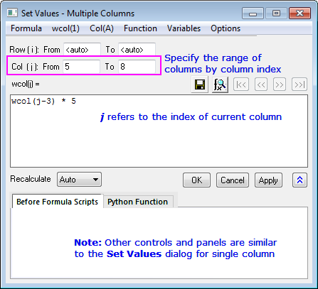
To open the Set Values dialog box for multiple columns:
| Menu Commands |
|
|---|---|
| Column Formula |
|
| Before Formula Scripts |
|
| Python Function |
|
|
Access to Origin's built-in functions:
|
To learn more, see Set Column Values - Quick Start
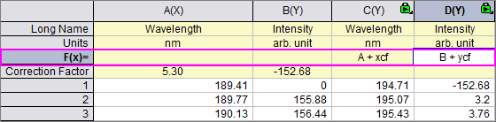
For simple expressions, you can use the F(x)= row to set column values. Any expression you enter here is directly entered into the Set Values dialog and vice versa. Note that the simplified spreadsheet cell notation that works in the formula box in Set Values also works in F(x)=:
Ease of use to the F(x)= label row:
|
Tutorial 1: A Quick Units Conversion using F(x)=
range r1=[F1]F1!wcol(j); //"j" is the column index.
range r2=[F2]F2!wcol(j);
|
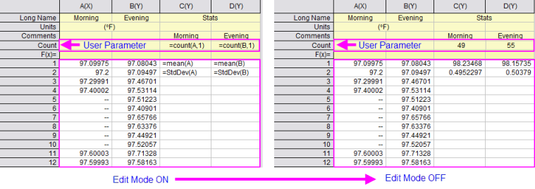
Origin supports cell-level expressions similar to those used by spreadsheet programs. Cell-level expressions which return a single value (numeric, string or date/time) can be entered into any worksheet data cell or into cells in a User-Defined Parameter row of the column label row area. When Edit Mode (Edit: Edit Mode) is toggled on, cell formulas display. When Edit Mode is toggled off, the formula result is displayed. Cell content can be edited regardless of Edit Mode state.
To learn more, see Using a Formula to Set Cell Values.
When creating cell formulas, or column formulas using F(x)=, the Formula Bar makes it easier to find and insert functions, select cell ranges and view and edit expressions, particularly long expressions that exceed cell width.
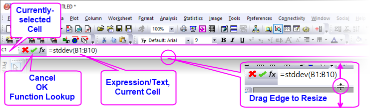
To enter an expression into a cell (data cell or F(x)=), click on the cell, then:
|
Note that you can drag the edge of the Formula Bar to resize it. You can also change the default font size by changing the value of LabTalk system variable @FBFS (default is "130"). |
|
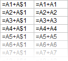
Tutorial 1: Extending a cell formula to other cells
|
|
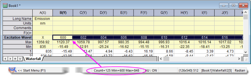
Tutorial 2: Quickly finding maximum values in multiple columns of data using special keyword "This" The only place where you can use cell formulas in the worksheet column label rows (worksheet header rows), is in a User Parameter row.
|
|
Tutorial 3: Use a column label row value in a cell calculation All data in the worksheet column label rows, including User Parameter rows, is stored as string data. To use a "number" stored in a column label row in a cell calculation, you must convert the string to a numeric value. In the following example, we use the LabTalk value() function to convert column label row data to a numeric so that it can be used in a cell calculation:
|
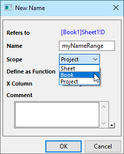
You can assign a name to a worksheet data range or column label rows, and use the name in cell formulas or column formulas and to define Reference Lines in graphs.
To create a named range:
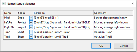
To manage named ranges:
Removing formulas and links can make it easier to share project data with colleagues without having to share such things as externally-linked (DDE) Excel files. It is also useful for significantly reducing project size before archiving data.
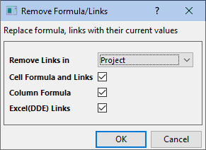
Things you can convert to raw numbers:
To open the tool:
for more information, see the Origin Help file.
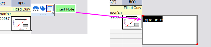
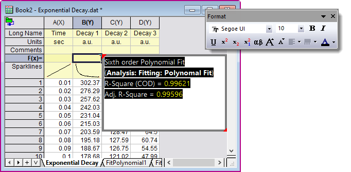
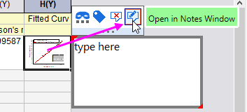
Any worksheet cell -- data row or column label row -- can contain a cell note; even those that contain data or other objects such as images or embedded graphs (Note: cells containing Links are not supported).
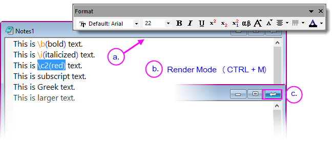
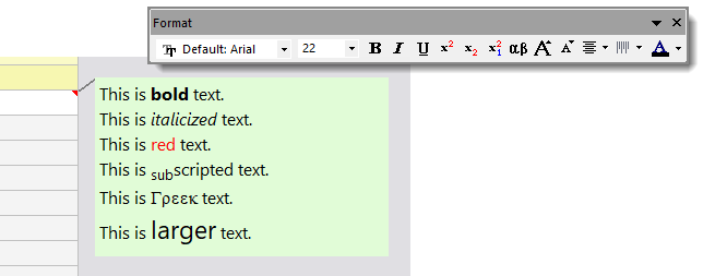
Worksheet cell Notes support Rich Text, meaning you can style text using Origin Rich Text syntax. In addition, you can add images and graphs, and link to worksheet cell values, report table values, etc. See Notes Windows for Reporting.
Notes:
|
In addition to styling text with the Format toolbar, you can apply a simple set of styles to each line/paragraph. Manage styles with the Text Styles Manager dialog box.
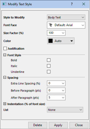
Note that you can add styles by selecting <new> from the Styles to Modify drop-down list; or select a style and Delete.
To apply a paragraph style to Notes window text:
Origin provides a number of utilities for manipulating worksheet data. Most of these are found on the Worksheet menu while some are on the Edit, Column or Analysis menus (note that a worksheet must be active). Some utilities are available from a shortcut menu: select your data and right-click.
| Utility | Menu Access |
|---|---|
|
Worksheet: Sort Range |
|
Edit: Find in Project |
|
Column: Hide/Unhide Columns |
|
Column: Move Columns or Column toolbar. |
|
|
|
|
|
|
|
Restructure: Join Worksheets by Column |
|
Restructure: Split Columns |
|
No menu access. To open the dialog box:
|
|
Restructure: Stack Columns |
|
|
|
Column: Filter menu, or Worksheet Data toolbar See Also: Data Masking |
|
Worksheet: Remove/Combine Duplicated Rows |
|
|
|
|
|
Worksheet: Conditional Formatting: Highlight |
|
Column: Reverse Order |
In addition to the above worksheet data utilities, the Origin worksheet supports Conditional Formatting. Conditional Formatting has three modes:
Manage conditional formatting in the active sheet using the Conditional Format Manager.
|
When using 3-Color Limited Mixing to apply color to worksheet heatmaps, you can now precisely control where the middle color falls. Specify by Percentile, by Percent or by Value. |
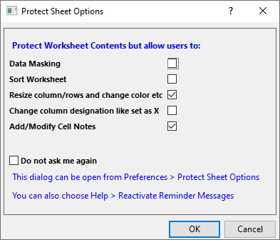
You can apply blanket protections to one or more worksheets and, in the process, provide for a few exceptions.
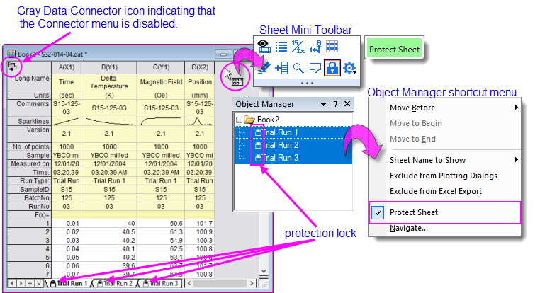
Any of these actions produces a Protect Sheet Options dialog so that you can set some exceptions. This dialog is also available by clicking Preferences: Protect Sheet Options.
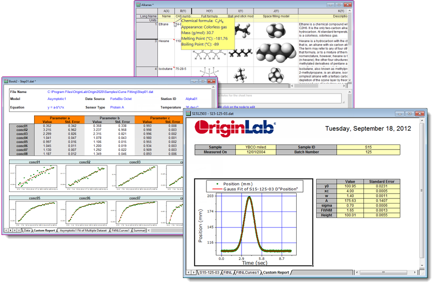
Apart from text and numeric data, the workbook can contain various other types of information -- images, graphs, notes and matrices; links to cell values in other books, project variables, documents or web pages; plus, import file metadata, variables and scripts -- making the workbook a flexible medium for collecting research data or for creating custom reports.
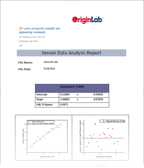
Further, as we will see, the workbook can "store" a complex sequence of analysis operations -- for instance, the application of a data filter, plus a fitting operation on the filtered data, combined with a customized plot of the results -- into something that we call an Analysis Template. The Analysis Template makes it possible to automatically generate a custom report of results, simply by supplying new input data.
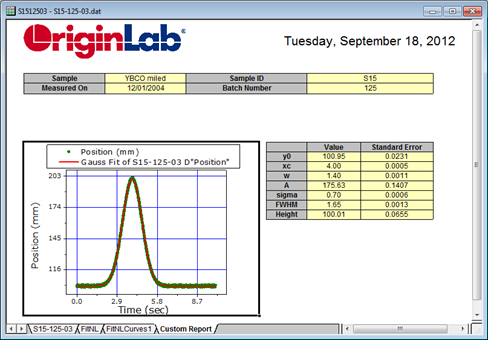
One attractive option for generating reports (there are others -- see the tip at the bottom of this section) is to export data to a custom MS Word template, and optionally, a PDF file. This is done by running an output-generating analysis in Origin, then associating key results with bookmarks in a Word template, and, finally, saving the workbook as an Analysis Template. To generate your report, you open the Batch Processing tool, point to both your Analysis Template and your Word template, run the batch process and generate your reports.
|
Another option for generating reports is to create HTML reports using Origin's Notes window. A Notes window can link to graphs, worksheet cells, etc., either directly or using a placeholder sheet. For more information, see HTML Reports from Notes Windows. |